SSC CGL Tier-II (JSO) 2022 Official Paper (Held On: 4 March 2023) (Previous Year Paper)

The correct answer is All of the options. 

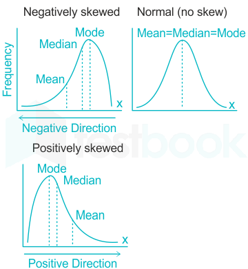
Key Points

• Tabulation refers to the systematic arrangement of data in columns or rows, usually in a tabular form, to facilitate analysis and comparison. It involves organizing and presenting data in a structured manner, making it easier to understand and draw conclusions from the information.
• Tabulation is commonly used in various fields, including statistics, research, surveys, and data analysis. It allows for the efficient representation of data, enabling individuals to summarize, analyze, and interpret information quickly and accurately.
• Merits of tabulation are: 
• Clarity and organization: Tabulation provides a clear and organized structure for presenting data. It helps to avoid clutter and confusion by systematically arranging information in columns and rows. This makes it easier for readers to understand and interpret the data.
• Easy comparison: Tabulation allows for the easy comparison of different variables or categories. By placing related information side by side, it becomes simpler to identify patterns, trends, and differences between data points. This aids in drawing meaningful insights and conclusions.
• Efficient data analysis: Tabulation facilitates data analysis by providing a concise summary of information. It allows researchers or analysts to perform calculations, statistical operations, and computations more efficiently. The organized format of the table simplifies complex calculations and enables quick data manipulation.
• Accessibility and readability: Tables are a widely understood and familiar format for presenting information. They provide a structured layout that is easily accessible to a wide range of audiences, including those who may not have in-depth knowledge of the subject matter. Tables also allow for the inclusion of headings, footnotes, and other explanatory notes, enhancing the readability and comprehension of the data.
• Visual representation: Tabulation offers a visual representation of data, which can make it easier to spot patterns and trends. By using elements like color coding, shading, or highlighting, tables can emphasize important information or draw attention to specific data points. This visual enhancement aids in quickly understanding and interpreting the data.
• Flexibility and adaptability: Tabulation allows for flexibility in the arrangement and organization of data. It can accommodate a wide range of variables, categories, and data types. Tables can be expanded or modified easily to include additional information or accommodate changing requirements, making them adaptable to different analytical needs.
• Effective communication: Tabulation is an effective means of communicating data and findings. It enables concise and structured reporting, making it easier for others to comprehend and utilize the information. Tables can be included in reports, presentations, research papers, or publications to convey data-driven insights in a clear and concise manner.

​Therefore, all of the above are the merits of data tabulation.

The correct answer is one year. 

Key Points

• In seasonal variations, the duration of time typically spans one year. Seasons are cyclical patterns that occur within a yearly cycle. They are influenced by factors such as the tilt of the Earth's axis and its orbit around the Sun.
• In most regions, the four primary seasons—spring, summer, autumn (fall), and winter—each last approximately three months. These seasons repeat annually, creating a predictable pattern of changes in temperature, weather conditions, and the growth and behavior of plants and animals.
• While there can be variations in the exact timing and intensity of seasons depending on the geographic location, the general timeframe of one year is typically used to define the duration of seasonal variations.
• For instance, temperatures over the course of five years can be observed to understand climate patterns, predicting weather conditions, and planning activities accordingly.

The correct answer is the coefficient of variation. 

Key Points 

• When a constant is added to each observation of a data set, the Coefficient of Variation (CV) will change.
• The Coefficient of Variation measures relative variability and is calculated as the ratio of the standard deviation to the mean, expressed as a percentage. Adding a constant to each observation will affect both the mean and the standard deviation. As a result, the ratio of the standard deviation to the norm, which is the Coefficient of Variation, will also change.
• The Coefficient of Variation is commonly used to compare the relative variability between different data sets or variables. When a constant is added to each observation, the relative variability, as measured by the Coefficient of Variation, will be altered. Therefore, the Coefficient of Variation will change when a constant is added to each observation in a data set.

Additional Information

• To calculate the Coefficient of Variation, divide the standard deviation by the mean and then multiply the result by 100 to express it as a percentage. The CV provides a relative measure of variability, allowing for comparison of the dispersion of different datasets or variables, regardless of their scales or units of measurement.
• CV = (Standard Deviation / Mean) * 100; Standard Deviation is the measure of dispersion that quantifies the average amount by which each data point varies from the mean. Mean is the average value of the data set. It is important to ensure that the mean and standard deviation are calculated based on the same set of data or population.

The correct answer is Repeated irregularly. 

Key Points 

• Seasonal variation is characterized by a repeated pattern within a specific time frame, typically one year. It follows a regular and predictable pattern as certain factors, such as the Earth's tilt and orbit around the Sun, influence the changes in weather, temperature, and other seasonal phenomena.
• The other statements are true for seasonal variation:
• Variation in a time series within one year: Seasonal variation refers to the changes or fluctuations observed in a time series data over a year.
• Caused by public holidays: Seasonal variation can be influenced by public holidays that occur at specific times of the year. These holidays often impact consumer behaviour, sales patterns, and other economic factors.
• Caused by rainfall: Seasonal variation can also be influenced by rainfall patterns. For example, some regions experience wet seasons and dry seasons, leading to variations in precipitation throughout the year. This, in turn, affects factors such as agricultural activities, water availability, and ecosystem dynamics.

Additional Information

• Seasonal variation is a fundamental aspect of many natural and human systems. It plays a crucial role in various fields such as meteorology, agriculture, economics, and tourism. Understanding and analyzing seasonal patterns are important for planning and decision-making in these domains.
• In meteorology, seasonal variation helps in predicting weather patterns and identifying climate trends.
• In agriculture, seasonal variation is crucial for crop planning, irrigation management, and pest control.
• In economics, seasonal variation affects consumer behaviour and spending patterns. Retailers, for example, rely on seasonal variations to plan their inventory, marketing campaigns, and sales strategies.
• In tourism, seasonal variation can have a significant impact on destination choices, travel patterns, and accommodation prices.
• Overall, seasonal variation provides valuable insights into the cyclical nature of various phenomena, allowing us to anticipate changes, make informed decisions, and adapt our activities accordingly.

The correct answer is $\rm r(X,Y)=\frac{Cov(X,Y)}{\sigma_X \sigma _Y}$. 

Key Points

• The Karl Pearson's correlation coefficient (r) between two random variables, X and Y, is computed using the formula:  $\rm r(X,Y)=\frac{Cov(X,Y)}{\sigma_X \sigma _Y}$
• Cov(X, Y) represents the covariance between variables X and Y. It measures how the variables vary together.
• σ_X is the standard deviation of variable X, which measures the variability or dispersion of X.
• σ_Y is the standard deviation of variable Y, which measures the variability or dispersion of Y.
• The correlation coefficient (r) measures the strength and direction of the linear relationship between X and Y. It ranges between -1 and 1, where:
• r = 1 indicates a perfect positive linear relationship, where X and Y increase or decrease together.
• r = -1 indicates a perfect negative linear relationship, where X and Y have an inverse relationship.
• r = 0 indicates no linear relationship between X and Y.
• The correlation coefficient not only provides information about the strength and direction of the relationship but also helps in assessing the degree to which X and Y vary together when compared to their individual variabilities (given by the standard deviations).

The correct answer is 6. 

Key Points

Five students failed the test. Their scores cannot be derived. But we can assume that one or more students might get the same marks.

Let's denote the test scores received by the failed students as F, where F = 0, 1, 2, 3. As the score of the students who passed the test starts from 4, F must be less than 4. 

Students who passed the test have scored 9, 6, 8, 7, 8, 9, 5, 6, 7 and 4. 

Arranging their scores in ascending order, we have: F, F, F, F, F, 4, 5, 6, 6, 7, 7, 8, 8, 9, 9 

n = total number of students = 15, an odd number. 

The median in the series would be $(n + 1) \over2$th term = (15 + 1) / 2 = 16 / 2 = 8^th number. 

The 8^th number in the series is 6.

The correct answer is R A Fisher 

Key Points 

• The analysis of variance (ANOVA) technique was developed by Ronald Aylmer Fisher, commonly known as R.A. Fisher. Fisher was a British statistician and geneticist who made significant contributions to the field of statistics, particularly in experimental design and inference.
• Fisher introduced the concept of variance analysis in his seminal work "The Design of Experiments" published in 1935. ANOVA is a statistical method used to analyze the differences between group means and determine whether these differences are statistically significant. It is widely used in various fields, including biology, psychology, social sciences, and engineering, to compare multiple groups or treatments.
• Fisher's work revolutionized the field of statistics and had a profound impact on experimental design, hypothesis testing, and data analysis. He received the Nobel Prize in Physiology or Medicine in 1938 for his contributions to the field of genetics and statistics.

Hence, the analysis of variance technique was developed by RA Fisher.

To find the value of A that minimizes the sum $\rm \Sigma_{i=1}^n(x_i-A)^2$, we need to find the value of A that minimizes the squared differences from the elements of series.

For the given series x₁, x₂, ...., x_n, the value of A that maximizes $\rm \Sigma_{i=1}^n(x_i-A)^2$, is the mean (average) of the series.

The given series is:

$\frac{1+2+3+4+5+6+7+8+9+10}{10}=\frac{55}{10}=5.5$

So the value of A that minimizes $\rm \Sigma_{i=1}^n(x_i-A)^2$= 5.5

The correct answer is (4.804, 5.196).

Key Points 

• In this scenario, we have a sample of 100 independent draws from a normal distribution with an unknown mean μ and a known variance σ^2 = 1. The sample mean is given as 5, which is the average of the 100 observed values.
• To estimate the population mean μ, we can construct a confidence interval. A 95% confidence interval means that if we were to take many random samples from the same population and calculate confidence intervals using the same method, approximately 95% of those intervals would contain the true population mean.
• The confidence interval (4.804, 5.196) represents the range of values that are estimated to contain the true population mean μ with 95% confidence. The lower bound of 4.804 indicates the lower end of the range, and the upper bound of 5.196 indicates the upper end of the range.
• Therefore, based on the given sample data and the properties of the normal distribution, we can be 95% confident that the true population mean μ falls within the interval (4.804, 5.196).
• This means that if we were to repeat the sampling process and calculate a new confidence interval each time, approximately 95% of those intervals would contain the unknown true population mean μ.

Additional Information

• (4.84, 6.196): The upper bound in this option is 6.196, which is outside of the plausible range for the population mean given the sample mean of 5. This interval is too wide and would lead to a wider range of values than what is expected with 95% confidence.
• (4.23, 5.19): The lower bound in this option is 4.23, which is lower than the plausible range for the population mean given the sample mean of 5. This interval is too narrow and would exclude potential values within the plausible range of the population mean with 95% confidence.
• (4.804, 6.196): The upper bound in this option is 6.196, which is outside of the plausible range for the population mean given the sample mean of 5. This interval is too wide and would lead to a wider range of values than what is expected with 95% confidence.

Hence, If the sample mean is 5, then the 95% confidence interval for μ is (4.804, 5.196).

The correct answer is 3, 300, 100 and 240  

Key Points

• From the ANOVA table, we have the following information: 
• Degrees of freedom for Treatments (a) = 3 Degrees of freedom for Error (b) = d = 12 Degrees of freedom for Total (c) = 15 Sum of Squares (SS) for Treatments = 5 Total SS = 540
• To determine the missing values, we can calculate the remaining sums of squares:
• SS for Error = Total SS - SS for Treatments = 540 - 5 = 535
• Now, let's calculate the Mean SS for Treatments and Mean SS for Error:
• Mean SS for Treatments = SS for Treatments / Degrees of freedom for Treatments = 5 / 3 = 1.67
• Mean SS for Error = SS for Error / Degrees of freedom for Error = 535 / 12 = 44.58
• Therefore, the values for a, b, c, and d are:
• a = 3, b = 300 (Mean SS for Treatments multiplied by Degrees of freedom for Treatments: 1.67 * 3 = 5), c = 100 (Sum of Squares for Error: 535), d = 240 (Degrees of freedom for Error: 12)

Hence, the values of a, b, c and d are, respectively, 3, 300, 100, and 240.

The correct answer is (- 10/9). 

Key Points

 Skewness (Sk) = ${(Mean - Mode)} \over S.D.$

The relationship between Standard Deviation (S.D) and Quartile Deviation (Q.D) is: $S. D. = {3\over 2}\times Q.D.$ 

Therefore, Skewness (Sk) = ${(Mean - Mode)} \over {{3\over 2} \times Q. D.}$Or, Sk = ${3 (2 - 7)} \over {{3\over 2} \times 3}$

Or, Sk = -10/9

Karl Pearson's coefficient of skewness is (-10/9). 

Important Points There are two formulas, that were developed by Karl Pearson, available to calculate the coefficient of skewness. One uses the mode while the other uses the mean. 

• Using Mean: Skewness (Sk) = ${(Mean - Mode)} \over S.D.$
• Using Median: Skewness (Sk) = ${3(Mean - Median)} \over S.D.$

The correct answer is average. 

Key Points

• Index numbers are a specialized average that are expressed in percentage form. They are commonly used to measure and compare changes in variables that are expressed in different units or have different scales of measurement. One of the main purposes of index numbers is to provide a relative measure of change over time. By selecting a base period and assigning it a value of 100, index numbers allow for easy comparison of subsequent periods to the base period.
• Here's how index numbers work:
• Selection of Base Period: A specific period is chosen as the base or reference period. The variables in subsequent periods will be compared to this base period.
• Calculation: The index number for each subsequent period is calculated by dividing the value of the variable in that period by the value in the base period and then multiplying by 100. This rescaling allows the index number to be expressed as a percentage relative to the base period.
• Interpretation: An index number above 100 indicates an increase or growth compared to the base period, while an index number below 100 indicates a decrease or decline.
• Index numbers have several advantages in measuring and comparing changes in variables expressed in different units:
• Standardization: Index numbers allow for the standardization of variables with different scales of measurement. By converting variables to a percentage-based index, they can be directly compared.
• Relative Comparison: Index numbers provide a relative measure of change, focusing on the percentage change rather than the absolute values. This allows for meaningful comparisons of variables over time.
• Comparison Across Categories: Index numbers can be used to compare changes across different categories or groups. For example, they can be used to compare price changes in different regions or the performance of different sectors in the economy.
• In summary, index numbers are a specialized average expressed in percentage form. They are used to measure and compare changes in variables that are expressed in different units or have different scales of measurement. They provide a standardized and relative measure of change, allowing for meaningful comparisons over time and across categories.

The correct answer is 0.3.

Key Points 

• The correlation coefficient between 2X and 3Y is also 0.3.
• When a variable is multiplied by a constant, such as multiplying X by 2 and Y by 3, it does not affect the correlation coefficient between the two variables. The correlation coefficient is not affected by the change of scale or origin.
• The correlation coefficient measures the strength and direction of the linear relationship between two variables, and scaling or multiplying the variables by a constant does not change that relationship.

Hence if the correlation between X and Y is 0.3, the correlation coefficient between 2X and 3Y would still be 0.3.

The correct answer is 12.5. 

Key Points Given,

The mean deviation of a set of observations (MD) is 15. 

MD = ${4 \over 5} σ$ , where $σ$ is the standard deviation 

Or, $σ = {4 \over 5} \times MD$ ______ (1)

The value of quartile deviation (QD) = ${2 \over 3} σ$ ________ (2)

Combining (1) and (2), QD $= {2 \over 3} \times {5 \over 4} \times 15$, as MD = 15 

Or, QD = 12.5 

Hence, the value of the quartile deviation is 12.5. 

The correct answer is ${10 \over 31}$

Key Points

 Given,

Envelope I contains 2 Black and 3 Red sheets while Envelope II contains 3 Black and 4 Red sheets. 

One envelope is selected at random and it is given probability of choosing envelope I is double that of envelope II. 

Let's denote the events of choosing envelopes I and II respectively as P(I) and P(II). 

As total probability is always 1, P(I) + P(II) = 1

Or, 2 P(II) + P(II) = 1 

Or, P(II) = 1/3 

Thus, P(I) = 2/3

The probability of choosing a red sheet from envelope I is P (R | I) = 3/5 and that from envelope II is P(R | II) = 4/7

According to Bayes' Theorem, the probability that the selected red sheet has come from envelope II is

= ${{P(II)} \times {P(R | II)} \over P(I) \times P(R | I) + P(II) \times P(R|II)}$

= ${{1 \over 3} \times {4 \over 7} \over {{2\over 3} \times {3 \over 5} + {4 \over 7} \times {1 \over 3}}}$

= $10 \over 31$

Hence, if a red sheet is drawn from the selected envelope, then the probability that it has come from envelope II is $10 \over 31$.

The correct answer is trend.

Key Points 

• The component containing the overall upward or downward pattern of the data in an annual time series is called the trend. The trend represents the long-term direction or movement in the data and helps identify whether the series is experiencing growth, decline, or remaining relatively stable over time.
• It captures the underlying systematic and persistent changes in the time series data, filtering out shorter-term fluctuations and random variations. Analyzing the trend can provide insights into the overall behaviour and direction of the data, which can be useful for forecasting and decision-making purposes.
• The trend can take various forms, depending on the nature of the data. It can be a linear trend, indicating a steady and consistent increase or decrease over time. For example, a linear upward trend might suggest a series experiencing continuous growth, while a linear downward trend might indicate a decline.
• The trend can also be nonlinear, exhibiting more complex patterns such as exponential growth or decay, cyclicality, or periodic fluctuations. Nonlinear trends may indicate seasonal or cyclical patterns within the data, where the series exhibits regular, repeating patterns over a specific period, such as monthly, quarterly, or annual cycles.
• Identifying and analyzing the trend is important in time series analysis and forecasting. It helps in understanding the overall behaviour and direction of the data, enabling the detection of long-term patterns, growth rates, and potential changes in the underlying dynamics.

Hence, the component containing the overall upward or downward pattern of the data in an annual time series is a trend.

The correct answer is symmetric. 

Key Points 

• Based on the given information that the 25^th, 50^th, and 75^th percentiles of a frequency distribution are equal to 2, 3, and 4, respectively, it suggests that the distribution is symmetric.
• In a symmetric distribution, the values are evenly distributed around the central point, which is typically the median (50^th percentile). If the 25^th and 75^th percentiles are equidistant from the median and have the same value difference, it indicates symmetry in the distribution.
• In this case, the difference between the 50^th percentile (median) and the 25^th percentile is 1 (3 - 2), and the difference between the 75^th percentile and the median is also 1 (4 - 3). This indicates that the values are symmetrically distributed around the median, with equal spread on both sides.

Therefore, based on the given percentiles, we can conclude that the distribution is symmetric.

The correct answer is Poisson Distribution 

Key Points 

• The distribution that exhibits the same mean and variance is the Poisson distribution. The Poisson distribution is commonly employed to model the occurrence of rare and independent events within a fixed time or space interval.
• Mathematically, the mean (μ) and variance (σ^2) in a Poisson distribution are equivalent: μ = σ².
• The probability mass function (PMF) of the Poisson distribution is defined as P(X=x)= ${e ^{-μ} μ^x} \over x!$where X represents a random variable following a Poisson distribution, x denotes the number of events, e is the base of the natural logarithm, and x! denotes the factorial of x.
• The Poisson distribution finds applications in various disciplines, including statistics, physics, biology, and telecommunications, particularly in scenarios where events occur randomly and possess a known average rate.

​

Additional Information

• The Poisson distribution finds applications in various disciplines, including statistics, physics, biology, and telecommunications, particularly in scenarios where events occur randomly and possess a known average rate.
• It is worth noting that the Poisson distribution assumes events to be independent and rare, meaning that the occurrence of one event does not influence the occurrence of another event, and the average rate of events remains constant throughout the interval.
• This distribution is widely used in analyzing phenomena such as the number of calls received by a call center within a specific time frame, the number of accidents occurring in a day, or the number of mutations in a DNA sequence.

The correct answer is (-1). 

Key Points

• Bowley's coefficient of skewness, also known as the quartile skewness coefficient, is a measure of skewness that compares the distance between the first quartile (Q1) and the median (Q2) with the distance between the median (Q₂) and the third quartile (Q₃) in a data set.
• The formula for Bowley's coefficient of skewness is: Sk = $(Q_1 - 2Q_2 + Q_3) \over (Q_3 - Q_1)$
• When the third quartile (Q₃) and the median (Q₂) are equal, the numerator of the formula becomes 0, resulting in a coefficient of skewness of -1. This indicates a perfectly negatively skewed distribution, where the data is concentrated on the right side of the median.
• In such a case, the data distribution has a longer tail on the left side, indicating that the majority of the data values are smaller than the median.
• It's important to note that Bowley's coefficient of skewness is just one measure of skewness and other measures such as the Pearson skewness coefficient or the moment coefficient of skewness may yield different results.

The correct answer is z-test. 

Key Points 

• If two large samples are drawn independently from two populations and we want to test the significance of the difference in proportions between the two populations, the appropriate test statistic is the Z-test.
• The Z-test is used to compare the difference between two proportions when the sample sizes are large. It is based on the assumption that the sampling distribution of the difference in proportions can be approximated by a normal distribution.
• The Z-test calculates the test statistic by comparing the observed difference in proportions to the expected difference under the null hypothesis. The test statistic is then compared to the critical value from the standard normal distribution to determine the statistical significance of the difference.
• The test statistic is a z-score (z) defined by the following equation is $z = {{(p−P)} \over σ}$; where, P is the hypothesized value of population proportion in the null hypothesis, p is the sample proportion and σ is the standard deviation of the sampling distribution.
• The formula for the Z-test statistic for comparing two proportions is $z = {{ ρ - P_0} \over \sqrt {P_0 (1 - P_0) \over n}}$ ; where, n = sample size, ρ = observed proportion and P0 is the null hypothesis.
• If the absolute value of the calculated Z-test statistic exceeds the critical value from the standard normal distribution, it indicates a significant difference between the two proportions.

Hence, in the case of testing the significance of the difference in proportions between two large independent samples, the appropriate test statistic is the Z-test.

The correct answer is 0.014. 

Key Points 

To calculate the probability that a randomly selected cellular call will have interference, the probabilities of selecting a call from each company and the probability of interference for each company are to be considered.

Given that Company A accounts for 60% (0.60) of the cellular phone market and 1% (0.01) of their calls have interference, and Company B accounts for 40% (0.40) of the market and 2% (0.02) of their calls have interference, we can calculate the overall probability of interference as follows:

Probability of interference

= (Probability of selecting Company A) × (Probability of interference in Company A) + (Probability of selecting Company B) × (Probability of interference in Company B)

= $(0.60 × 0.01) + (0.40 × 0.02)$

= 0.006 + 0.008

= 0.014

Hence, the probability that a randomly selected cellular call will have interference is 0.014

The correct answer is $\rm \Sigma_{j=1}^k n_j(\bar x_{j}- \bar x)^2$. 

 Key Points

• The sum of squares due to treatments (SST) in a completely randomized design can be calculated using the formula: $\rm \Sigma_{j=1}^k n_j(\bar x_{j}- \bar x)^2$
• Σk represents the sum of the k treatments. It indicates that we consider each treatment separately.
• Σj=1nj represents the sum of the observations within each treatment. It implies that we calculate the sum of squares for each treatment individually.
• x̅j is the mean of the jth treatment, which represents the average value of the response variable for that particular treatment.
• x̅ is the grand mean, which represents the overall average value of the response variable across all treatments and observations.
• To calculate the SST, we take the difference between each treatment mean (x̅j) and the grand mean (x̅). We square this difference to eliminate any negative signs and emphasize the magnitude of the difference. We then sum up these squared differences across all treatments and observations.
• The resulting SST value reflects the total variation in the response variable that can be attributed to the differences between the treatment means. It represents the variability between treatments and is used to assess the significance and effectiveness of the different treatments in the study.
• By comparing the SST to other sums of squares, such as the sum of squares due to error (SSE) or the total sum of squares (SSTotal), we can further analyze and interpret the effects of treatments on the response variable.

Hence, the required formula is $\rm \Sigma_{j=1}^k n_j(\bar x_{j}- \bar x)^2$

The correct answer is $\rm \frac{Mean-Mode}{Standard\ deviation}$ . 

 Key Points

• Karl Pearson's measure of skewness, also known as Pearson's first skewness coefficient, is defined as the ratio of the third moment about the mean to the cube of the standard deviation. It is calculated using the following formula:
• Pearson's skewness coefficient = $\rm \frac{Mean-Mode}{Standard\ deviation}$
• To be more precise, Pearson's skewness coefficient measures the degree and direction of skewness in a distribution. The numerator, which is the difference between the mean and mode, captures the direction of skewness. A positive value indicates a right-skewed distribution, where the tail is elongated towards higher values. A negative value indicates a left-skewed distribution, where the tail is elongated towards lower values.
• Dividing the numerator by the denominator, the standard deviation, scales the skewness measure and makes it independent of the scale of the data.
• It's important to note that there are other measures of skewness as well, such as the Fisher-Pearson skewness coefficient and the Bowley skewness coefficient, which may have slightly different formulas and interpretations.

Hence, Karl Pearson’s measure of relative skewness is $\rm \frac{Mean-Mode}{Standard\ deviation}$

The correct answer is $\rm d\frac{n(n+1)}{2n+1}$ 

Key Points 

• For the arithmetic series a, a + d, a + 2d, ..., a + 2^nd, the mean deviation from the mean can be calculated using the formula:
• Mean deviation from the mean = $\rm d\frac{n(n+1)}{2n+1}$; where, d is the common difference between terms in the series, n is the number of terms in the series.
• The formula you provided calculates the mean deviation from the mean for an arithmetic series. It takes into account the common difference (d), the number of terms (n), and the mathematical relationship to determine the average deviation from the mean.
• This formula is derived by summing the deviations of each term from the mean, considering the pattern and structure of the arithmetic series. The resulting expression provides a concise way to calculate the mean deviation from the mean for such a series.

The correct answer is watching movies. 

Key Points

 Data collection methods typically involve systematic approaches to gathering information or data from various sources. Examples of commonly used data collection methods include surveys, interviews, observations, experiments, questionnaires, and focus groups. These methods are designed to collect specific data or information relevant to a research or study objective. Watching movies, on the other hand, is a leisure activity or form of entertainment and does not typically involve collecting structured data or information for research purposes.

Additional Information

• ​Interviews are a data collection method where researchers directly interact with participants to gather information. This can be done through face-to-face conversations, phone calls, or virtual meetings. Interviews provide an opportunity to ask open-ended or structured questions, allowing for an in-depth exploration of the topic. Researchers can probe for detailed responses, gain insights into participants' perspectives, and collect qualitative data. Interviews are valuable for obtaining rich, nuanced data and establishing a deeper understanding of the research subject.
• Questionnaires involve presenting participants with a set of pre-designed questions to collect information. They can be administered in written or electronic format. Questionnaires often use closed-ended questions with predefined response options, facilitating standardized data collection. They are efficient for gathering data from large samples and enabling quantitative analysis. Questionnaires allow researchers to collect data on attitudes, opinions, behaviours, and demographics. Careful design ensures clarity, relevance, and proper sequencing of questions for reliable and valid data collection.
• Surveys are a widely used data collection method that involves gathering information from a large population or sample. Surveys typically employ structured questionnaires to collect data on specific topics of interest. They can be administered through various channels, including online platforms, email, or paper-based forms. Surveys enable researchers to collect quantitative data, analyze patterns, and draw statistical conclusions. They offer a cost-effective and efficient way to obtain data from a diverse range of participants and are suitable for a wide range of research objectives.

The correct answer is Median. 

Key Points

• The median divides an observation into two equal parts. The median is a measure of central tendency that represents the middle value of a dataset when the values are arranged in ascending or descending order. In other words, it is the value that separates the higher half of the observations from the lower half.
• By definition, 50% of the observations fall below the median, and 50% fall above it. Therefore, the median divides the dataset into two equal parts, making it a useful measure for understanding the central position of the data.

Additional Information

• When analyzing data, understanding the central tendency is crucial in capturing the essence of the dataset. While the mean is a widely used measure, there is another valuable measure called the median.
• The median plays a unique role in providing insights into the distribution and central position of the data. Unlike the mean, which is influenced by extreme values, the median offers a robust alternative that is less affected by outliers.
• By dividing the dataset into two equal parts, the median serves as a powerful tool for understanding the typical value or observation at the center. Whether working with numerical or ordinal data, the median proves versatile, making it valuable in a wide range of fields such as statistics, economics, and social sciences.

The correct answer is 3. 

Key Points 

• If the fourth central moment of a mesokurtic distribution is 243 and the standard deviation is 3, we can calculate the variance and confirm if it aligns with a mesokurtic distribution.
• The fourth central moment (μ₄) is related to the variance (σ²) as follows: μ₄ = σ⁴(κ + 3) - 3σ⁴
• For a mesokurtic distribution, the kurtosis (κ) is 3. Substituting the given values into the equation, we have: 243 = 3⁴(3 + 3) - 3(3⁴) 243 = 81(6) - 3(81) 243 = 486 - 243 243 = 243
• Since the equation holds true, we can conclude that the variance is indeed 243. Taking the square root of the variance, we find: σ = √243 σ = 3

Hence, the standard deviation is 3.

The correct answer 12^th observation in the series after arranging in ascending order. 

Key Points

The method to determine the third quartile of a series with 15 observations is as follows: 

• First, we need to find the position of the third quartile using the formula:
• Position of the third quartile = (3/4) * (n + 1); where n represents the total number of observations. In this case, n is 15.
• Plugging in the values, we have: 
• Position of the third quartile = (3/4) * (15 + 1) = (3/4) * 16 = 12
• The position of the third quartile is 12.
• Next, we arrange the series in ascending order and locate the value at the 12^th position. This observation represents the third quartile. (Alternatively, if the series is already sorted in ascending order, the third quartile will be the 12^th observation directly.)

Hence, in both cases, the third quartile will be equal to the 12^th observation in the series after arranging it in ascending order.

The correct answer is Mean = Median = Mode

Key Points 

• The property that the mean, median, and mode are equal in a normal distribution is a fundamental characteristic of its symmetrical shape.
• In a normal distribution, the data is symmetrically distributed around the mean, creating a bell-shaped curve. The mean represents the arithmetic average of the data points, indicating the central tendency of the distribution.
• The median, on the other hand, represents the middle value that divides the distribution into two equal halves. The mode refers to the value that occurs most frequently in the dataset.
• Since the normal distribution is symmetric, with equal proportions of data on both sides of the mean, the median and mode coincide with the mean. This means that the central value of the distribution, which represents the peak or highest point, is also the value that occurs most frequently and divides the data into equal halves.
• The equality of the mean, median, and mode in a normal distribution simplifies the understanding and analysis of the data. It provides a reference point for locating the center of the distribution and understanding the typical value that represents the dataset.
• This property also facilitates various statistical calculations and inference procedures based on the normal distribution, as it allows for simpler computations and interpretations.

• Hence, the fact that the mean, median, and mode are equal in a normal distribution is true.

The correct answer is 26.

Key Points

• The residual degrees of freedom represent the number of observations in the data that are free to vary after accounting for the differences between the groups. These degrees of freedom are used to estimate the variability within each group and the overall error or residual variability in the ANOVA analysis.
• To calculate the residual or error degrees of freedom in a one-way ANOVA with three groups, we follow a step-by-step method. 
• Determine the total sample size: Add up the number of observations in each group. In this case, we have 10 + 9 + 10 = 29 observations.
• Identify the number of groups: In a one-way ANOVA, we compare the means of different groups. Here, we have three groups.
• Calculate the residual degrees of freedom: Subtract the number of groups from the total sample size. In this case, the calculation is 29 - 3 = 26.
• Having 26 residual degrees of freedom means that there are 26 independent pieces of information available to estimate the error variability in the model.
• This information is crucial for conducting hypothesis tests and making inferences about the differences between the group means in the ANOVA analysis.

The correct answer is $\rm \frac{m(m^2-1)}{12}$

Key Points

• The correction factor required to be added in the calculation of Spearman's rank correlation when 'm' individuals receive the same rank is given by the formula: $\rm \frac{m(m^2-1)}{12}$, where, 'm' represents the number of individuals who have the same rank in the data set.
• The correction factor is used to adjust for tied ranks in the calculation of Spearman's rank correlation coefficient. When there are ties in the ranks, it means that multiple individuals have the same rank value. The correction factor takes into account the extent of these ties and helps in providing a more accurate estimate of the rank correlation.
• By adding the correction factor to the rank correlation formula, we account for the impact of tied ranks on the final correlation coefficient. This ensures that the rank correlation calculation appropriately reflects the strength of the relationship between the variables, considering the ties in the data.
• Including the correction factor is important in situations where ties occur in the data set, as it helps to improve the accuracy and validity of the Spearman's rank correlation coefficient as a measure of association between variables.

Additional Information

• Spearman's rank correlation coefficient, named after Charles Spearman, is a non-parametric measure of correlation between two variables. It is based on the ranks of the observations rather than their actual values.
• Spearman's rank correlation is widely used in various fields, such as social sciences, economics, psychology, and biological research. It provides a robust and flexible measure of association between variables, particularly when the data does not meet the assumptions of parametric correlation measures like Pearson's correlation coefficient.

The correct answer is $\rm \frac{2r^2}{1+r}$

Key Points 

• The formula for the multiple correlation coefficient (R) = $\rm \frac{2r^2}{1+r}$
• In this formula, r represents the pairwise correlation coefficient between any two variables, such as r12 for X1 and X2, r13 for X1 and X3, and r23 for X2 and X3.
• The multiple correlation coefficient measures the strength of the linear relationship between the dependent variable (Y) and the set of independent variables (X1, X2, X3) collectively. It indicates how well the independent variables, taken together, predict the variation in the dependent variable.
• The value of R ranges from 0 to 1, where 0 indicates no linear relationship and 1 indicates a perfect linear relationship between the variables. A higher value of R suggests a stronger correlation and implies that the independent variables jointly explain more of the variance in the dependent variable.
• The formula calculates the multiple correlation coefficient based on the pairwise correlation coefficients. It shows the relationship between the individual pairwise correlations (r) and the overall multiple correlations (R), highlighting the combined effect of the variables on the dependent variable.

Additional Information

• The multiple correlation coefficient is commonly employed in regression analysis. It helps evaluate the overall goodness of fit of the regression model and assess the strength of the relationship between the independent variables and the dependent variable when multiple predictors are involved.
• While the formula assumes equal pairwise correlations (r), in practice, the actual values of the pairwise correlations can vary, and more advanced methods may be required to estimate the multiple correlation coefficient accurately.

The correct answer is 70^th percentile

Key Points 

• In statistics, percentiles are a way to divide a dataset into hundred equal parts based on their relative rank or position. Each percentile represents a specific percentage of the data below it. For example, the 70^th percentile signifies that 70% of the observations in the dataset are less than or equal to the value at that percentile.
• Deciles, on the other hand, divide the dataset into ten equal parts. Each decile represents a specific range of percentiles. The 7^th decile corresponds to the range of percentiles from the 60^th to the 70^th.
• When we say that the 7^th decile is equivalent to the 70^th percentile, it means that the value at the 70^th percentile acts as the boundary value between the 6^th and 7^th deciles. This boundary value represents the value below which 70% of the data falls.
• By utilizing percentiles and deciles, we can analyze the distribution of data, identify specific ranges of values, and determine the relative position of individual observations within the dataset in a more formal and structured manner.

The correct answer is $13 \over 18$.

Key Points 

To find the probability $P ({1 \over 3} \leq x \leq {4 \over 3})$ using the given probability density function (pdf), we need to integrate the pdf over the specified range.

The pdf $f(x) = 1 - |1 - x|$ is a piecewise function. Let's split the integration into two parts: 

For $0 < x < 1$: 

$f(x) = 1 - (1 - x) = x$

For $1 \leq x < 2$ :

$f(x) = 1 - |1 - x| = 1 - (x - 1) = (2 - x)$

Now, we can evaluate the probability: $P ({1 \over 3} \leq x \leq {4 \over 3}) = \int\limits_{1\over 3}^{4\over3} f(x) dx$

Evaluating the integrals: \([{x^2\over2}]{1\over3}^{1} + [2x - {x^2\over 2}]{1}^{4\over3}\)

Simplifying this, we have: $({1\over 2} - {1\over 18}) + ({8 \over 3} - {8\over 9} - 2 + 1) = {13\over 18}$

Hence, the required probability is $13\over 18$.

The correct answer is $227 \over 144$ 

Key Points To calculate the variance of a discrete random variable, you can use the following formula: $Var(X) = E[(X - \mu)^2]$ and the mean = $\mu = E(X) = \sum X_i P(X_i)$; where E represents the expected value and μ represents the mean of the random variable X, P(X_i) represents the probabilities corresponding to each X_i

Hence, the mean $\mu = - {11\over 12}$

Hence, the variance of X = Var(X) = $227\over 144$

The correct answer is symmetric and platykurtic 

Key Points

• Based on the provided information regarding the first four central moments of a distribution:
• μ1 = 0 μ2 = -93 μ3 = 0 μ4 = 2.53
• We can deduce the following characteristics of the distribution:
• Symmetry: The fact that the first central moment (μ1) is zero indicates that the distribution possesses symmetricity. A zero value for μ1 suggests that the distribution is centred around its mean, implying the absence of skewness.
• Kurtosis (Platykurtic): The positive value of the fourth central moment (μ4) at 2.53 implies positive kurtosis. Positive kurtosis suggests that the distribution possesses heavier tails and a more peaked shape than a normal distribution. Specifically, the given value of μ4 indicates a platykurtic distribution, signifying lighter tails and a flatter peak compared to a normal distribution.

Hence, based on the provided information, the distribution can be formally described as symmetric and platykurtic.

The correct answer is $\rm \frac{\Sigma ip_{1ii}q_{0i}}{\Sigma ip_{0i}q_{0i}}$. 

Key Points 

• The formula for calculating Laspeyres' index number, using the usual notations, is as follows:
• Laspeyres' Index = $\frac{\Sigma ip_{1ii}q_{0i}}{\Sigma ip_{0i}q_{0i}}$; where  
• $\Sigma$ indicates the summing operation.
• $i$ represents the index of the individual items or categories being considered.
• $p_{1ii}$ refers to the current period (usually denoted as period 1) price of item i.
• $p_{0i}$ represents the base period (usually denoted as period 0) price of item i.
• $q_{0i}$ denotes the base period quantity of item i.
• To calculate Laspeyres' index, we sum up the products of the current period price, $p_{1ii}$, and the base period quantity, $q_{0i}$, for each item or category. Then, divide this sum by the sum of the products of the base period price, $p_{0i}$, and the base period quantity, $q_{0i}$, for each item or category.
• This index is commonly used to measure the change in the value of a specific set of goods or items between two periods, with the base period as the reference point.

Additional Information

• Laspeyres' index number compares the value or quantity of goods or items in a current period (period 1) with the value or quantity of the same goods or items in a base period (period 0). It is a fixed-base index, meaning that the base period remains constant throughout the analysis.
• Laspeyres' index number is often used in economics, particularly in price index calculations, to measure the change in the cost of a fixed basket of goods over time. It is useful for analyzing inflation, as it provides a measure of the average price change for a specific set of goods or items.
• It's important to note that Laspeyres' index has some limitations, including potential substitution bias and not capturing changes in consumption patterns. Other index number formulas, such as Paasche's index and Fisher's index, address these limitations by considering different weighting schemes or using average prices from both periods.

Overall, index numbers, including Laspeyres' index, are valuable tools for analyzing changes in variables over time and making meaningful comparisons.

The correct answer is 11. 

Key Points 

• Given that the fourth central moment of a frequency distribution is equal to 11, denoted as μ4 = 11, and all odd raw moments are zero, we can derive information about the distribution's characteristics. 
• First, the fourth central moment measures the shape and spread of the distribution, particularly its kurtosis. A positive value of μ4 indicates that the distribution has heavier tails and a more peaked shape compared to a normal distribution.
• Additionally, when all odd raw moments are zero, it implies that the distribution exhibits symmetry. Symmetry means that the distribution is balanced around the origin and does not display any skewness.
• Since we have a symmetric distribution with μ4 = 11, it follows that the fourth raw moment, denoted as m4, is also equal to 11. In symmetric distributions, the central moments and raw moments of the same order are equal. Therefore, if the fourth central moment is 11, it implies that the fourth raw moment is also 11.
• In summary, based on the assumption that μ4 = 11 and all odd raw moments are zero, we can formally conclude that the fourth raw moment of the frequency distribution, m4, is equal to 11.

The correct answer is the coefficient of variation. 

Key Points

Coefficient of variation:

The coefficient of variation (CV) is a statistical measure that expresses the standard deviation as a percentage of the mean. It is calculated by dividing the standard deviation by the mean and multiplying by 100. The CV provides a relative measure of dispersion because it considers the standard deviation in relation to the mean. It is commonly used when comparing the variability of different datasets with different means. 

Additional Information

• Quartile deviation: The quartile deviation measures the spread or dispersion of a dataset by calculating the difference between the upper quartile (Q3) and the lower quartile (Q1). However, it does not provide a relative measure of dispersion since it is an absolute measure that does not take into account the magnitude of the data values.
• Harmonic mean: The harmonic mean is a measure of central tendency and does not directly measure dispersion. It calculates the reciprocal of the average of the reciprocals of a set of values. It is primarily used to calculate rates or averages in cases where the data values have a reciprocal relationship, such as rates of speed or time.
• Standard deviation: The standard deviation is a measure of dispersion that quantifies the amount of variation or spread in a dataset. It measures the average distance of data points from the mean. While the standard deviation provides an absolute measure of dispersion, it does not directly provide a relative measure unless it is compared to the mean or other reference values.

Hence the coefficient of variation is the measure of relative dispersion.

The correct answer is θ.

Key Points

• The mode of a probability distribution is the value of the random variable where the probability density function (pdf) reaches its maximum. The pdf for the random variable X given here is a continuous function on the interval [0, θ], and is 0 everywhere else.
• This particular pdf is a monotonically increasing function of x on the interval [0, θ] (since x^2 is an increasing function on [0, θ] and θ^2 is a positive constant). This means that the function f(x) increases as x increases within this interval.

Hence, the mode of X, the point where the pdf f(x) is at its maximum, is at x = θ.

The correct answer is 0.204 

Key Points 

• The exponential distribution has a probability density function (pdf) given by $f(x; λ) = λe^{(-λx)}$ for x ≥ 0 and λ > 0. The rate parameter λ is the parameter we want to estimate.
• The method of maximum likelihood estimation (MLE) is commonly used for this purpose. The likelihood function for a sample {x₁, x₂, ..., x_n} drawn from an exponential distribution is given by: $L(λ; x_1, x_2, ..., x_n) = λn \times e^{(-λ \sum x_i)}.$
• Taking the natural logarithm gives the log-likelihood function, which simplifies the process of finding the maximum: $l(λ; x_1,X_2, ..., x_n) = n log (λ) - λ \sum x_i$
• To find the maximum likelihood estimate, we differentiate this function with respect to λ, set the derivative equal to zero, and solve for λ. This gives: 

${d \over dλ} [l (λ; x_1, x_2, ..., x_n)] = {n \over λ} - \sum x_i = 0$

• Rearranging this gives the maximum likelihood estimate for λ: $λ̂ = {n \over \sum x_i}$
• For the given sample {1, 3, 1, 8, 2, 8, 3, 8, 2, 13}, we have n = 10 (the number of observations) and ∑x_i = 1 + 3 + 1 + 8 + 2 + 8 + 3 + 8 + 2 + 13 = 49.
• Plugging these into the formula gives: $λ̂ = {10 \over 49} \approx 0.204$

The maximum likelihood estimate of the rate parameter λ for the given sample is approximately 0.204.

The correct answer is all observations are equal.  

Key Points

• The mean absolute deviation (MAD) is a measure of dispersion that calculates the average absolute difference between each data point and the mean of the dataset.
• Among the alternatives provided, the mean absolute deviation (MAD) is zero when all observations are equal.
• In a dataset where all observations are equal, the absolute difference between each data point and the mean will be zero for every observation. When calculating the average of these zero differences, the result will also be zero.

Additional Information

• When all observations are different from each other:
• In this scenario, the MAD will not be zero. Since all observations are different, there will be non-zero absolute differences between each data point and the mean. When averaged, these non-zero differences will result in a non-zero MAD.
• When few observations are equal to one and few are equal to two:
• In this scenario, the MAD will not be zero either. As there are different values present in the dataset (one and two), the absolute differences between each data point and the mean will be non-zero. Averaging these non-zero differences will lead to a non-zero MAD.
• When few observations are zero and few are non-zero:
• Similar to the previous scenarios, the MAD will not be zero in this case. Since there are both zero and non-zero values in the dataset, the absolute differences between each data point and the mean will be non-zero. Computing the average of these non-zero differences will yield a non-zero MAD.
• When all observations are equal:
• When all observations in a dataset are equal, the absolute difference between each data point and the mean will be zero for every observation. Consequently, when averaging these zero differences, the result will be zero. Thus, in this scenario, the MAD will be zero.

Hence, when all observations in a dataset are equal, the mean absolute deviation (MAD) will be zero.

The correct answer is It is expensive. 

Key Points 

Non-probability sampling represents a set of sampling techniques where the samples are assembled in a manner that does not afford all individuals in the population an equal chance of selection. Here are evaluations of the proposed statements: 

• Non-probability sampling is a fast method: This statement is generally accurate. Non-probability sampling can frequently be executed more swiftly than probability sampling because it doesn't necessitate the establishment of a comprehensive sampling frame that enumerates every individual in the population.
• Non-probability sampling is expensive: This statement is typically incorrect. Methods involving non-probability sampling are usually less financially demanding than those employing probability sampling. This is because they can be carried out more promptly and do not necessitate interaction with every individual in the population.
• Non-probability sampling employs a subjective approach in sample selection: This statement is correct. Given that non-probability sampling does not provide every individual in the population an equal opportunity of being chosen, it is frequently perceived as a more subjective technique. The investigator utilizes their discretion to select participants, which could lead to bias.
• Non-probability sampling is an easy method: This statement is generally accurate. Techniques involving non-probability sampling are often less complex to carry out than those involving probability sampling because they do not necessitate a comprehensive list of the population or intricate random selection procedures.

In conclusion, the assertion that does NOT hold for non-probability sampling is the second statement: "Non-probability sampling is expensive." Contrarily, non-probability sampling techniques are generally less costly than probability sampling methods.

The correct answer is 18/19. 

Key Points

The probability function delineated describes a discrete random variable, denoted as X, which can assume the values 0.5, 1, and 10 with corresponding probabilities of 18/38, 18/38, and 2/38 respectively. The probability that X resides within the range from 0 to 2, which can be denoted as P(0 ≤ X ≤ 2), is obtained by summing the probabilities corresponding to the values X=0.5 and X=1. This can be computed by adding the probabilities p(0.5) and p(1) as follows: 

P(0 ≤ X ≤ 2)

= p(0.5) + p(1)

= 18/38 + 18/38

= 36/38 = 18/19. 

Hence, the probability that X is within the range from 0 to 2, P(0 ≤ X ≤ 2), is indeed equal to 18/19.

The correct answer is 1/2

Key Points 

The probability density function (pdf) of a continuous random variable integrates to 1 over its entire domain. In this case, the pdf is defined on the interval [0,3). We can therefore determine the value of a by setting up and solving the following integral: 

$\rm\displaystyle \int_0^3p(x)dx=1$

or, $\rm\displaystyle \int_0^1a(x)dx+\rm\displaystyle \int_1^2adx+\rm\displaystyle \int_2^3(-ax+3a)dx=1$

or, $\rm a\times \frac{1}{2}[x^2]_0^1+ax[x]_1^2+(-a)\frac{1}{2}[x^2]_2^3+3a[x]_2^3=1$

or, $\rm \frac{a}{2}+a(2-1)+\frac{(-a)}{2}(3^2-2^2)+3a(3-2)=1$

or, $\rm \frac{a}{2}+a-\frac{5a}{2}+3a=1$

or, $\rm \frac{a+2a-5a+6a}{2}=1$

or, 9a - 5a = 2

or, 4a = 2

or, $\rm a=\frac{2}{4}=\frac{1}{2}$

Hence, the correct value of 'a' is 1/2.

The correct answer is $\rm \mu_4=\mu^{'}_4-4\mu_3^{'}\mu_1^{'}+6\mu_2^{'}(\mu_1^{'})^2-3(\mu_1^{'})^4$

Key Points

Let μ_4 denote the fourth-order moment about the origin, and $μ'_1, μ'_2, μ'_3$ represent the first, second, and third raw moments about the origin, respectively. Furthermore, let μ symbolize the mean of the random variable. 

• The equation provided is: $μ_4 = μ'_4 - 4μ'_3μ'_1 + 6μ'_2(μ'_1)^2 - 3(μ'_1)^4$; where, 
• $μ_4$ represents the expected value of the random variable raised to the power of 4, adjusted by subtracting the fourth power of the mean.
• $μ'_4$represents the expected value of the random variable raised to the power of 4 without adjusting for the fourth power of the mean.
• $μ'_3$ represents the expected value of the random variable raised to the power of 3 without adjusting for the cube of the mean.
• $μ'_1$represents the expected value of the random variable without adjusting for the mean.
• $μ'_2$represents the expected value of the random variable squared without adjusting for the square of the mean.

This equation illustrates the relationship between these moments, demonstrating how the fourth-order moment about the origin can be computed based on the raw moments and the mean. It is important to note that this equation assumes a symmetric distribution, where the central moments and raw moments are equivalent. For distributions that are not symmetric, the equation may differ or involve additional terms.

The correct answer is 1. 

Key Points 

Given the observations 2, 3, 5, 6, x, 8, 9, to determine the median, we arrange the observations in ascending order: 2, 3, 5, 6, x, 8, 9. 

Since the number of observations is odd, the median is the middle value in the ordered list. In this case, the fourth observation, which is 6, represents the median.

• To identify the values that x cannot be equal to, we need to consider the possible positions of x in the ordered list. 
• If x is less than 6, it would be positioned to the left of 6 in the list. In such a case, the median would be greater than 6, as the middle value would shift to a higher number. Therefore, x cannot be less than 6.
• If x is greater than 6, it would be positioned to the right of 6 in the ordered list. In this case, the median would still be 6 since it represents the middle value. Therefore, x can be greater than 6.
• If x equals 6, it would coincide with the median, as it represents the middle value in the ordered list. Therefore, x can be equal to 6.

Hence, considering the given information that the median is known to be 6, it can be concluded that x cannot be equal to 1, as it is less than 6.

The correct answer is 0.032

Key Points 

In multiple correlations, the correlation between two variables is denoted by the subscripted notation "r_xy," where x and y represent the variables involved. In this case, "r₁₂" represents the correlation between variables 1 and 2, while "r₂₁" represents the correlation between variables 2 and 1.

Since correlation measures the linear relationship between two variables, it follows that "r₁₂" is equal to "r₂₁." The correlation between variables 1 and 2 is the same as the correlation between variables 2 and 1. Thus, "r₁₂" can indeed be equal to "r₂₁" in multiple correlations. 

Here,  r12 = 0.7, r13 = 0.72 and r23 = 0.52 can be interpreted as  r21 = 0.7, r31 = 0.72 and r23 = 0.52

Now, 

$\rm r_{23.1}=\frac{r_{23}-r_{21}r_{31}}{\sqrt{\left(1-r_{21}^2\right)\left(1-r_{31}^2\right)}}$

r₁₂ = r₂₁ = 0.7

r₁₃ = r₃₁ = 0.72

r₂₃ = 0.52

$\rm r_{23.1}=\frac{0.52-0.7\times 0.72}{\sqrt{(1-0.7^2)(1-0.72^2)}}$