Concept:
Convolution of a signal x(t) with unit impulse δ(t) is the signal itself. i.e. x(t) ⊕ δ(t) = x(t)
Fourier transform of auto-correlation function of a power signal x(t) is power spectral density Sx(f). i.e. RX(τ)↔FTSX(f)
And E(x2 (t)) = RX (0)
The variance of the signal x(t) is defined as:
var(x(t))=E(x2(t))−(E(x(t))2
Fourier transform of unit impulse is 1.
δ(t)↔FT1
Calculation:
Let n(t) be the input white noise with zero mean and 2N0 power spectral density.
Mean of the white noise = E(n(t)) = 0
Power spectral density is:
Sn(f)=2N0 ;
And the auto-correlation function is:
Rn(τ)↔FTSn(f)
2N0→IFT2N0δ(t)
Rn(τ)=2N0δ(t)
Let yn(t) is the output noise.

Mean of the output noise:
\( = E\left( {{y_n}\left( t \right)} \right) = E\left( {n\left( t \right) \times \mathop \smallint \nolimits_{ - \infty }^\infty h\left( t \right)dt} \right)\)
\( = E\left( {n\left( t \right)} \right) \times \mathop \smallint \nolimits_{ - \infty }^\infty h\left( t \right)dt\)
\( = 0 \times \mathop \smallint \nolimits_{ - \infty }^\infty h\left( t \right)dt = 0\)
The variance of the output noise is:
Var(yn(t))=E(yn2(t))−(E(yn(t))2
=E(yn2(t))
E(yn2(t))=Ryn(0)
\({R_{{y_n}}}\left( \tau \right) = h\left( \tau \right){h^}\left( { - \tau } \right)*{R_n}\left( \tau \right)\)
\( = \left( {\mathop \smallint \nolimits_{ - \infty }^\infty h\left( t \right).h\left( {t + \tau } \right)dt} \right)*\frac{{{N_0}}}{2}{\rm{\delta }}\left( {\rm{\tau }} \right)\)
\( = \left( {\mathop \smallint \nolimits_{ - \infty }^\infty h\left( t \right).h\left( {t + \tau } \right)dt} \right) \times \frac{{{N_0}}}{2};\)
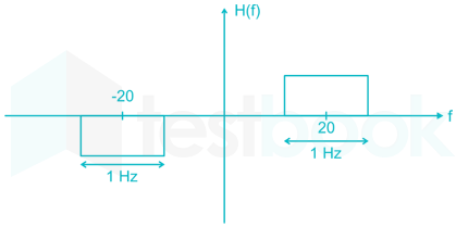
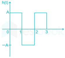
\({R_{{y_n}}}\left( 0 \right) = \left( {\mathop \smallint \nolimits_{ - \infty }^\infty h\left( t \right).h\left( t \right)dt} \right)\frac{{{N_0}}}{2} = \left( {\mathop \smallint \nolimits_{ - \infty }^\infty {h^2}\left( t \right)dt} \right)\frac{{{N_0}}}{2} = 3{A^2} \times \frac{{{N_0}}}{2}\)
Var(yn(t))=23A2.N0