GATE EC 2014 Official Paper: Shift 4 (Previous Year Paper)

The correct answer is option 1), i.e. dissent.

Key Points 

Let's try to find the meaning of words given in the options-

• Dissent: (noun) the holding or expression of opinions different from those commonly or officially held. (आम तौर पर या आधिकारिक तौर पर आयोजित विचारों से अलग राय की होल्डिंग या अभिव्यक्ति)
• Descent: (noun) an act of moving downwards, dropping, or falling. (नीचे की ओर बढ़ने, गिरने या गिरने की क्रिया)
• Decent: (adjective) of an acceptable standard; satisfactory. (एक स्वीकार्य मानक का; संतोषजनक।)
• Decadent: (adjective) characterized by or reflecting a state of moral or cultural decline. (नैतिक या सांस्कृतिक गिरावट की स्थिति को दर्शाती या दर्शाती है।)

The given sentence mentions the freedom of a citizen to disagree with the government, the only option 1), i.e. dissent would be apt.

The correct answer is option 2), i.e. get back to him. 

Revert: (verb) to reply or respond to someone. It also means to return to a previous state, practice, topic, etc. 

Let's look at the other words given in the options:

• Retract: draw or be drawn back or back in.
• Retreat: withdraw from enemy forces as a result of their superior power or after a defeat.

The correct answer is option 2), i.e. vindicated. 

Vindicated: (adjective) justified, cleared of blame. 

Let us try to find the meaning of other words given in the options- 

• Punished: (verb) inflict a penalty or sanction on someone for an offence. It is the past and the past participle form of "punish".
• Substantiated: (verb) proved the truth by giving evidence. It is the past and the past participle form of "substantiate".
• Appreciated: (verb) recognized the full worth of. It is the past and the past participle form of "appreciate".
• Chastened: (verb) to inflict suffering upon for purposes of moral improvement. It is the past and the past participle form of "chasten".

The only word similar in meaning to "vindicated" is "substantiated", i.e. option 2).

Given:

P = xⁿy^m

Now x^’ = 2x, y^’ = y/2

∴ P^’ = (x^’)ⁿ(y^’)^m

P^’ = (2x)ⁿ(y/2)^m

^{\(P' = {\left( {2x} \right)^n}{\left( {\frac{y}{2}} \right)^m} = {2^n}{\left( {\frac{1}{2}} \right)^m}\left( {{x^n}{y^m}} \right) = {2^{n - m}}P\)}

Hence, option 1 is the correct answer.

Concept:

In a consecutive series

\(\frac{{sum,of,numbers}}{{total;numbers}} = middle;number;of;the;series\)

Calculation:

As 425 is the sum of the first 5 consecutive odd numbers

∴ \(\frac{{425}}{5}\) = 85 is the middle of 5 numbers i.e. 3^rd number.

∴ Series is 81, 83, 85, 87,…….101, 103

Sum of last 5 number is 95 + 97 + 99 + 101 + 103 = 495

Explanation:

Sequence is 13 + 4 = 17, 17 + 2 =19, 19 + 4 = 23

M + 4 = Q, Q + 2 = S, S + 4 = W

According to the given code, only consonants are taken and written in reverse order.

KCLFTSB: BST - Best, F - Of, LCK - Luck

SHSWDG: GD - Good, WSHS - Wishes

Similarly

“ace the Exam": C - Ace, T - The, XM - Exam

Concept:

As the increase in annual rate is uniform over time.

∴ it is a case of compound interest.

\(A = P{\left( {1 + \frac{R}{{100}}} \right)^t}\)

where A = amount, P = principle, R = rate, t = time

Calculation:

Given:

A = 2P

\(A = P{\left( {1 + \frac{R}{{100}}} \right)^t}\)

\(2P = P{\left( {1 + \frac{R}{{100}}} \right)^{10}}\)

\({\left( {1 + \frac{R}{{100}}} \right)^{10}} = 2\)

\({\left( {1 + \frac{R}{{100}}} \right)^{10}} = 2\)

R = 7.17 ≃ 7.2 %

\(Total;% ;,increase = \frac{{3660000 - 3000000}}{{3000000}} \times 100 = \frac{{660000}}{{3000000}} \times 100 = 22;% \)

Explanation:

The digit in unit place is selected in 4! Ways

The digit in tens place is selected in 4! Ways

The digit in hundreds place is selected in 4! Ways

The digit in the thousand's place is selected in 4! Ways

The digit in ten thousand's place is selected in 4! Ways

Sum of all values for 1

4! × 1 × (10⁰ + 10¹ + 10² + 10³ + 10⁴)

= 4! × 11111 × 1

Similarly for ‘3’ = 4! × (11111) × 3

Similarly for ‘5’ = 4! × (11111) × 5

Similarly for ‘7’ = 4!× (11111) × 7

Similarly for ‘9’ = 4!× (11111) × 9

∴ sum of all such number = 4! × (11111) × (1 + 3 + 5 + 7 + 9) = 24 × (11111) × 25 = 6666600

Given:

Expanding the given expression, we can write:

\(\mathop \sum \limits_{n = 0}^\infty \frac{1}{{\angle n}} = 1 + \frac{1}{{\angle 1}} + \frac{1}{{\angle 2}} + \frac{1}{{\angle 3}} + \frac{1}{{\angle 4}} + \ldots \)

\(\mathop \sum \limits_{n = 0}^\infty \frac{1}{{\angle n}} = 1 + 1 + \frac{1}{2} + \frac{1}{6} + \frac{1}{{24}} + \ldots \)    --- (1)

The series expansion of exponential function is given by:

\({e^x} = 1 + x + \frac{{{x^2}}}{{\angle 2}} + \frac{{{x^3}}}{{\angle 3}} + \frac{{{x^4}}}{{\angle 4}} + \ldots \)

\({e^x} = 1 + x + \frac{{{x^2}}}{2} + \frac{{{x^3}}}{6} + \frac{{{x^4}}}{{24}} + \ldots \)

Putting x = 1

\({e^1} = e = 1 + 1 + \frac{1}{2} + \frac{1}{6} + \frac{1}{{24}} + \ldots \)    ---(2)

From (1) and (2), we get:

\(e = \mathop \sum \limits_{n = 0}^\infty \frac{1}{{\angle n}}\)

Or

\(\mathop \sum \limits_{n = 0}^\infty \frac{1}{{\angle n}} = e\)

Hence option 4 is correct.

Concept:

The gradient in all coordinate system is defined below:

Calculation:

Given V = 𝑥² + 3𝑦² + 𝑧³ and

the point is (x, y, z) = (1, 1, 1)

from V, a_x = x², a_y = 3y², a_z = z³

\(\nabla V=\frac{{\partial \left( {{{\rm{x}}^2}{\rm{;}} + {\rm{;}}3{{\rm{y}}^2}{\rm{;}} + {\rm{;}}{{\rm{z}}^3}{\rm{;}}} \right)}}{{\partial x}}{a_x} + \frac{{\partial \left( {{{\rm{x}}^2}{\rm{;}} + {\rm{;}}3{{\rm{y}}^2}{\rm{;}} + {\rm{;}}{{\rm{z}}^3}{\rm{;}}} \right)}}{{\partial y}}{a_y} + \frac{{\partial \left( {{{\rm{x}}^2}{\rm{;}} + {\rm{;}}3{{\rm{y}}^2}{\rm{;}} + {\rm{;}}{{\rm{z}}^3}{\rm{;}}} \right)}}{{\partial z}}{a_z}\)

\(\nabla V=2x{a_x} + 6y{a_y} + 3{z^2}{a_z}\)

The magnitude of the gradient is:

\(\sqrt {V_x^2 + V_y^2 + V_z^2} \)

gradient at (x, y, z) = (1, 1, 1) is

 \(2 \times 1{a_x} + 6 \times 1{a_y} + 3 \times {1^2}{a_z}\)

∴ The magnitude is:

\(\sqrt {{2^2} + {6^2} + {3^2}} \)

\( = \sqrt {4 + 36 + 9} \)

 \( = \sqrt {49} = 7\)

Extra Information:

Del operator: It is written ∇, is the differential operator. In cartesian coordinates, it is defined as:

\(\nabla = \frac{\partial }{{\partial x}}{a_x} + \frac{\partial }{{\partial y}}{a_y} + \frac{\partial }{{\partial z}}{a_z}\). The letters in the bold represent vectors

The operator is useful in defining

• The gradient of a scalar V, written as ∇ V
• The divergence of a vector A, written as ∇ ⋅ A
• The curl of a vector A, written as ∇ × A
• The Laplacian of a scalar V, written as ∇ 2 V

​The Del operator in all coordinates are mentioned below:

\(\rho = \sqrt {{x^2} + {y^2} } \) and

\(tan\phi = \frac{y}{x}\)

\(r = \sqrt {{x^2} + {y^2} + {z^2}} \) and

\(tan\theta = \frac{{\sqrt {{x^2} + {y^2}} }}{z}\)

The Gradient of a scalar field V is a vector that represents both magnitude and the direction of the maximum space rate of increase in V

Grad V = ∇ V = \(\frac{{\partial V}}{{\partial x}}{a_x} + \frac{{\partial V}}{{\partial y}}{a_y} + \frac{{\partial V}}{{\partial z}}{a_z}\)

ax, ay, az are unit vectors along x, y, z directions.

Physical significance:

1. Gives a vector normal to surface taken at point P

2. It gives the direction of the maximum rate of change of function

3. Directional derivatives of a scalar function at the same point ‘P’ in the direction of the vector \(\vec a\) is given by (grad V)P⋅ and unit  vector defined as \(\hat a = \frac{{\vec a}}{{\left| {\vec a} \right|}}\)

Concept:

A Gaussian random variable X with mean μ and variance σ² can be denoted as X N (μ, σ²) and its probability density function (pdf) is given by:

\({f_x}\left( x \right) = \frac{1}{{\sqrt {2\pi {\sigma ^2}} }}{e^{ - {{\left( {x - \mu } \right)}^2}/2{\sigma ^2}}}\)

The expectation of any function of x is calculated as:

\(E\left[ {g\left( x \right)} \right] = \mathop \smallint \limits_{ - \infty }^\infty g\left( x \right) \cdot {f_x}\left( x \right)dx\)

If f(-x) = f(x) then f(x) is said to be even function of x.

And, an even function satisfies:

\(\mathop \smallint \limits_{ - \infty }^\infty f\left( x \right)dx = 2\mathop \smallint \limits_0^\infty f\left( x \right)d\tau \)

Calculation:

Given:

X ∼ N (0, 1)

\({f_X}\left( x \right) = \frac{1}{{\sqrt {2\pi } }}{e^{ - {x^2}/2}}\)

\(E\left[ {\left| X \right|} \right] = \mathop \smallint \limits_{ - \infty }^\infty \left| x \right|;{f_X}\left( x \right)dx\)

\( = \mathop \smallint \limits_{ - \infty }^\infty \left| x \right| \cdot \frac{1}{{\sqrt {2\pi } }}{e^{ - {x^2}/2}}dx;\)

\(= \frac{1}{{\sqrt {2\pi } }}\mathop \smallint \limits_{ - \infty }^\infty \left| x \right| \cdot {e^{ - {x^2}/2}}dx\)

Since:

\(\left| x \right| \cdot {e^{ - {x^2}/2}}\) is an even function of ‘x’, we can write:

\(E\left[ {\left| x \right|} \right] = \frac{1}{{\sqrt {2\pi } }} \times 2\mathop \smallint \limits_0^\infty x \cdot {e^{ - {x^2}/2}}dx\)

Using substitution of variables:

\(Let;\frac{{{x^2}}}{2} = y\)

\(x;dx = dy\)

\(E\left[ {\left| x \right|} \right] = \frac{1}{{\sqrt {2\pi } }} \times 2\mathop \smallint \limits_0^\infty {e^{ - y}}dy\)

\( = \sqrt {\frac{2}{\pi }} ;{ - {e^{ - y}}\left. \right|_0^\infty = \sqrt {\frac{2}{\pi }} ;\left{ {1 - 0} \right}\)

\(E\left[ {\left| x \right|} \right] = \sqrt {\frac{2}{\pi }} \simeq 0.798\)

E[|x|] ≃ 0.8

Concept:

Differential equation: It is an equation which involves differential coefficients or differentials.

The solution of differential equations consists of two parts Complementary function (C.F) and Particular Integral (P.I)

To solve the linear second-order differential equation which is in a general form as shown:

  \(\frac{{{d^n}y}}{{d{x^n}}} + {k_1}\frac{{{d^{n - 1}}y}}{{d{x^{n - 1}}}} + {k_2}\frac{{{d^{n - 2}}y}}{{d{x^{n - 2}}}} + \cdots + {k_n}y = 0\)

 this equation in symbolic form is

\(\left( {{D^n} + {k_1}{D^{n - 1}} + \cdots + {k_n}} \right)y = 0\)

We assume operator ‘D’ as d/dx and form auxiliary Equation.

To find the roots of the differential equation, make symbolic coefficient to zero.

  \({D^n} + {k_1}{D^{n - 1}} + \cdots + {k_n} = 0\) is called auxiliary equation and (A.E.)

Let m₁, m₂, ⋯ , m_n be its roots.

There are four different types of roots.

1. If roots are different m₁ ≠ m₂ then solution is of the form

\({c_1}{e^{{m_1}x}} + {c_2}{e^{{m_2}x}} \)

2. If the roots are equal, m₁ = m₂ = m

\(\left( {{c_1} + {c_2}} \right){e^{mx}} \)

3. If the roots are complex and not equal m₁ = α + ι β and m₂ = α - ι β

\({e^{\alpha x}}\left( {{C_1}cos\beta x + {C_2}sin\beta x} \right) \)

4. If roots are complex and equal, i.e**, m₁ = m₂ = α + ι β and m₃ = m₄ = α - ι β**

\({e^{\alpha x}}\left( {\left( {{c_1}x + {c_2}} \right)cos\beta x + \left( {{c_3}x + {c_4}} \right){\bf{cos\beta x}}} \right) \)

P.I part is also found in different methods based on the X function which is R.H.S of differential function.

Calculation:

Given DE is \(\frac{{{d^2}x}}{{d{t^2}}} + 2\frac{{dx}}{{dt}} + x = 0\) 

A.E is D² + 2D + 1 = 0 and roots of AE are (D+1)(D+1) = 0

so roots are equal and m = -1

∴ from the above table we can write the solution for given equation as

 \(\left( {a + bt} \right){e^{mt}} = \left( {a + bt} \right){e^{ - t}}\)

Concept:

Direction derivative at any point (x, y) is defined as:

\(\nabla f \cdot \hat n{\left. \right|_{at\left( {x,y} \right)}}\)

Where,

∇f = gradient of given function

n̂ = direction vector.

Calculation:

\(f = \frac{{xy}}{{\sqrt 2 }}\left( {x + y} \right)\)

\(f = \frac{{{x^2}y}}{{\sqrt 2 }} + \frac{{x{y^2}}}{{\sqrt 2 }}\)

The unit vector at an angle of π/4 with y-axis will be:

\(\hat n = \frac{1}{{\sqrt 2 }}{a_x} + \frac{1}{{\sqrt 2 }}{a_y}\)

\(\nabla f = \frac{{\partial f}}{{\partial x}}{a_x} + \frac{{\partial f}}{{\partial y}}{a_y}\)

\(\nabla f = \left( {\frac{{2 x y + {y^2}}}{{\sqrt 2 }}} \right){a_x} + \left( {\frac{{2xy + {x^2}}}{{\sqrt 2 }}} \right){a_y}\)

\(\nabla f \cdot \hat n = \left( {\frac{{2xy + {y^2}}}{2}} \right) + \left( {\frac{{2xy + {x^2}}}{2}} \right)\)

\(\nabla f \cdot \hat n{\left. \right|_{\left( {1,1} \right)}} = \frac{{2 + 1}}{2} + \frac{{2 + 1}}{2}\)

\( = \frac{3}{2} + \frac{3}{2} = 3\)

Concept:

There are two kinds of voltage or current sources:

Independent Source: It is an active element that provides a specified voltage or current that is completely independent of other circuit variables.

Dependent Source: It is an active element in which the source quantity is controlled by another voltage or current in the circuit.

Analysis:

Let R_L be the load, and the current through it will be I_L.

\({I_L} = \frac{{ - {A_i}{I_i}R}}{{R + {R_L}}}\)

I_L ∝ I_i

Since output current is proportional to input current, it is a current-controlled current source.

Concept:

Substitution Theorem states that if an element in a network is replaced by a voltage/current source whose voltage/current at any instant of time is equal to the voltage/current across the element in the previous network then the initial condition in the rest of the network will be unaltered.

Additional Information

Substitution Theorem:

• It is applicable for any linear bilateral network consisting of a number of energy sources with passive elements.
• Any passive element can be substituted in terms of equivalent voltage (or) current and vice versa for further analysis and reduction in the network without disturbing the remaining network.
• Power absorbed by this passive element, and its equivalent substitution voltage / current source remains the same.

Calculation:

Using the substitution theorem, we can replace the current source in parallel to the resistance with a voltage source in series with an equivalent resistance.

For the given circuit, we do the following transformation:

The given circuit is redrawn as:

Applying KVL through the loop, we get:

20 – 2kI – Ik – 4kI + 8 – 3kI = 0

28 = 10 k × I

I = 2.8 mA

Concept:

The frequency and wavelength are related by the relation:

\(\nu =\frac{c}{λ}\)

Less the wavelength more will be the frequency and vice-versa.

Also, the energy of a photon with wavelength λ is given by:

\(E= \frac{{hc}}{\lambda}\)

To generate electron-hole pairs, the energy of the incident photon must be greater than the Band-gap energy.

Application:

The wavelength of the incident radiation of energy 1.42 eV will be:

\(λ = \frac{{hc}}{E}\)

\( \lambda= \frac{{6.62 \times {{10}^{ - 34}} \times 3 \times {{10}^8}}}{{1.42 \times 1.6 \times {{10}^{ - 19}}}}\)

\(\lambda = 0.87 \times {10^{ - 6}};m\)

\(\lambda = ;0.87;\mu m\)

So, the radiation of wavelength less than 0.87 μm can generate electron-hole pair in Ga As, as the frequency will be more.

∴ Option (1) best satisfies the required condition.

Concept:

We know that the conductivity of Intrinsic semiconductor is given by:

σ_i = n_i q (μ_n + μ_p)

Also, the intrinsic carrier concentration is defined as:

\({n_i} = \sqrt {{A_0}} {T^{\frac{3}{2}}}{e^{ - {E_{G0}}/2KT}}\)

The intrinsic conductivity will be:

\({\sigma _i} = \sqrt {{A_0}} {T^{3/2}}{e^{ - {E_{G0}}/2KT}}q\left[ {{\mu _n} + {\mu _p}} \right]\)

Also, we know that:

\({\mu _n} \propto {T^{ - \frac{3}{2}}}\) and \({\mu _p} \propto {T^{ - \frac{3}{2}}}\)

\({\mu _n} = {\mu _{n0}}{T^{ - \frac{3}{2}}}\) and \({\mu _p} = {\mu _{{p_0}}}{T^{ - \frac{3}{2}}}\)

The conductivity Equation (1) can now be written as:

\({\sigma _i} = \sqrt {{A_0}} {e^{ - {E_{G0}}/2KT}}q{T^{\frac{3}{2}}}\left[ {\mu_{n_0} + \mu_{p_0}} \right]{T^{ - 3/2}}\)

\({\sigma _i} = \sqrt {{A_0}} {e^{ - {E_{G0}}/2KT}}q\left[ {{\mu _{{n_0}}} + {\mu _{{p_0}}}} \right]\)

Since the Resistivity is the inverse of conductivity, we can write:

\({p_i} = \frac{1}{{{\sigma _i}}}\)

\({p_i} = \frac{1}{{\sqrt {{A_0}} {e^{ - {E_{G0}}/2KT}}q\left( {\mu_{n_0} + \mu_{p_0}} \right)}}\)

\(ln{p_i} = ln1 - ln\left[ {\sqrt {{A_0}} {e^{ - \frac{{{E_{G0}}}}{{2KT}}}}V\left( {{\mu _{{n_0}}} + {\mu _{{p_0}}}} \right)} \right]\)

\(ln{p_i} = 0 - \left[ {ln\sqrt {{A_0}} - \frac{{{E_{G0}}}}{{2KT}} + lnV\left( {{\mu _{{n_0}}} + {\mu _{{p_0}}}} \right)} \right]\)

\(ln{p_i} = \frac{{{E_{G0}}}}{{2K}}\frac{1}{T} + ln\left[ {\sqrt {{A_0}} V\left( {{\mu _{{n_0}}} + {\mu _{{p_0}}}} \right)} \right]\)

Comparing this with the equation of the line: y  = m x + C, we get the slope as:

\(m = \frac{{{E_{G0}}}}{{2K}}\) = Band Gap energy of silicon.

Concept:   \(\rm \lambda = \frac{{hc}}{{{E_g}}}\)

Application: As we know

\(\rm \lambda = \frac{{hc}}{{{E_g}}}\)

\(\rm = \frac{{6.62 \times {{10}^{ - 34}} \times 3 \times {{10}^8}}}{{1.1 \times 1.6 \times {{10}^{ - 19}}}}\)

\(\rm = 1.128 μm\)

The circuit diagram of a Common-emitter amplifier without a bypass is drawn as:

Voltage gain is given by:

\(\frac{{{V_0}}}{{{V_i}}} = \frac{{ - {g_m}{R_i}'}}{{1 + {g_m}{R_E}}}\)

Where R_L’ = R_L’||R_E

And the circuit diagram of a common emitter amplifier with bypass is drawn as:

Voltage gain is given by:

\(\frac{{{V_o}}}{{{V_i}}} = - {g_m}{R_i}'\)

Where, R_L’ = R_C||R_L

Input resistance, R_i = r_x

Observation: Clearly, the voltage gain decreases, and the input resistance is increased if the emitter is not bypassed.

Try to solve all the diode related questions with the following approach:

1. Consider all the diodes to be off.

2. Now, first, calculate the voltage across each diode.

3. If the diodes have greater voltage than cut-in voltage, consider that the diode to be on which has higher voltage.

4. Now, again calculate the voltage across the remaining diode by considering that particular diode to be ON.

5. Again check which diode has a greater voltage considering it ON, and the process continues till we get to know the state of each diode.

Analysis:

Given: V_r = 0.7 V

When V_i > 2.7 V, the output voltage will be fixed to:

V₀ = 2.7 V

When V_i < -1.7 V, the output voltage will again be fixed to:

V₀ = -1.7 V

When -1.7 V < V_i < 2.7 V, both the diodes are OFF and:

V₀ = V_i

∴ The transfer characteristics can be drawn as:

Analysis:

Given: 

V⁺ = V_A and V^- = V_Z

When V_i acts as a trigger to change the output state, the capacitor C₁ changes until the output state returns to the original state.

Initially, the capacitor is uncharged.

Let V₀ = + V_sat

Now, the voltage across capacitor is given by:

V_l(t) = V_f + (V_i - V_f) e^{-t / τ}

With V_i = 0 V and V_f = +V_sat, we can write:

\({V_c}\left( t \right) = {V_{sat}} + \left( {0 - {V_{sat}}} \right){e^{ - t/{R_1}{C_1}}}\) 

\({V_c}\left( t \right) = {V_{sat}}\left( {1 - {e^{ - \frac{t}{{{R_1}{C_1}}}}}} \right)\) 

\({V_c}\left( t \right) = {V_{sat}} - {V_{sat}}{e^{ - t/{R_1}{C_1}}}\) 

\({V_{sat}} - {V_c}\left( t \right) = {V_{sat}}{e^{ - t/{R_1}{C_1}}}\)    ---(1)

From the given figure:

V₀ – V_c(t) – V_A = 0 and V₀ = V_sat

V_sat – V_c(t) – V_A = 0

V_sat – V_c(t) = V_A  ---(2)

From (1) & (2), we get:

\({V_A} = {V_{sat}};{e^{ - t/{R_1}{C_1}}}\) 

Let the trigger input applied, be in the triangular, i.e.

With \(;{V_Z} = \frac{{d{V_i}}}{{dt}}:\)

Now, 

Hence a pulse of short duration is generated with the help of a trigger input.

∴  It is a monostable multivibrator.

Concepts:

Generally, a sample & hold circuit is designed using an opamp. The given circuit shows the general implementation:

Sample & Hold circuit capacitor C_H is charged by the AmplifierA₁.

The maximum output current of the opamp is given as:

\({I_{max}} = {C_H} \times \left( {\frac{{d{V_o}}}{{dt}}} \right)\)

Droop rate = \(\frac{{d{V_o}}}{{dt}}\), when V₀ is the voltage at the steady state.

The acquisition time (t_ac) is depicted in the following figure:

Analylsis:

\({I_{max}} = {C_H} \times \left( {\frac{{d{V_o}}}{{dt}}} \right)\)

\({I_{max}} = ;{C_H} \times \left( {\frac{{d{V_o}}}{{dt}}} \right) = Constant\)

If C­_H increases then ‘t’ which is the acquiring time must also increase to maintain the relationship.

Also, capacitor discharging time constant T_C(discharge) is proportional to capacitance i.e.

\({T_{{C_{discharge}}}} \propto {C_H}\)

So if C_H increases then capacitor voltage decreases slowly because of discharging time constant, this means droop rate decreases.

The given circuit is redrawn as:

The output will be:

\(Y = \overline {\left( {\overline {A + B} } \right) + AB} \)

\(Y = \overline {\bar A\bar B + AB} \)

\(Y = \overline {A \odot B} \)

Y = A ⊕ B

Y = A̅ B + A B̅ 

Additional Information

All Boolean algebra laws are shown below

Concept:

• The given circuit contains both NMOS and PMOS. So it is a CMOS implementation.
• For CMOS implementation if NMOS transistors are in series then PMOS transistors corresponding to their NMOS counterparts will be in parallel.
• Similarly, if NMOS transistors are in parallel then PMOS transistors corresponding to their NMOS counterparts will be in series.
• The output will be the negate of the function implemented by the NMOS transistors.

According to De morgan's theorem:

\(\overline {{A_1}.{A_2} \ldots \ldots {A_n}} = \overline {{A_1}} + \overline {{A_2}} + \ldots \overline {{A_n}} \)

Calculation:

In the given circuit, signals A, B, and C̅  are in series for NMOS implementation. ∴ The output will be:

\(\left( Y \right) = \overline {A.B.\bar C} = \bar A + \bar B + C\)

Concept:

The Fourier transform of aⁿu(n) is given as:

\({a^n}u\left( n \right)\mathop \leftrightarrow \limits^{F.T.} \frac{1}{{1 - a{e^{ - j\omega }}}}\)

Also, the time-shifting property of Fourier transforms states that:

If x(n) ↔ X(jω)

\(x\left( {n - {n_0}} \right) \leftrightarrow {e^{ - j{n_0}\omega }} \cdot X\left( {j\omega } \right)\)

Application:

Let \(f\left( n \right) = {\left( {\frac{2}{3}} \right)^n}u\left( n \right)\)

The Fourier Transform of f(n) will be:

\(F\left( {j\omega } \right) = \frac{1}{{1 - \left( {\frac{2}{3}} \right){e^{ - j\omega }}}}\)

Replacing ‘ω’ with 2nf, we get:

\(F\left( f \right) = \frac{1}{{1 - \left( {\frac{2}{3}} \right){e^{ - j2\pi f}}}}\)

Applying Time shifting property, we can write:

\({\left( {\frac{2}{3}} \right)^{n + 3}}u\left( {n + 3} \right) \leftrightarrow \frac{{{e^{j \cdot 3\omega }}}}{{1 - \left( {\frac{2}{3}} \right){e^{ - j2\pi f}}}}\)

The above expression can be written as:

\({\left( {\frac{2}{3}} \right)^3} \cdot {\left( {\frac{2}{3}} \right)^n}u\left( {n + 3} \right) \leftrightarrow \frac{{{e^{j \cdot 6\pi f}}}}{{1 - \left( {\frac{2}{3}} \right){e^{ - j2\pi f}}}}\)

Multiplying both sides with \({\left( {\frac{3}{2}} \right)^3}\), we get:

\({\left( {\frac{2}{3}} \right)^n}u\left( {n + 3} \right) \leftrightarrow \frac{{{{\left( {\frac{3}{2}} \right)}^3} \cdot {e^{j6\pi f}}}}{{1 - \left( {\frac{2}{3}} \right){e^{ - j2\pi f}}}}\)

Comparing this with the given transform, we get:

\(A = {\left( {\frac{3}{2}} \right)^3} = {\left( {1.5} \right)^3}\)

A = 3.375

Concept:

Time-shifting property of Fourier Transform:

Shiting in time domain results in a phase shift in the frequency domain, i.e.

\(If;x\left( t \right)\mathop \leftrightarrow \limits^{FT} X\left( f \right)\)

\(x\left( {t - {t_0}} \right)\mathop \leftrightarrow \limits^{FT} X\left( f \right){e^{ - j2\pi f{t_0}}}\)

If a signal x(t) is passed through a system having transfer function H(f), then the output of the system is:

\(Y\left( f \right) = X\left( f \right)H\left( f \right)\)

where \(x\left( t \right)\mathop \leftrightarrow \limits^{FT} X\left( f \right)\) and

\(y\left( t \right)\mathop \leftrightarrow \limits^{FT} Y\left( f \right)\)

Calculation:

Since both X(f) and H(f) are band-limited to the same frequency band, we can write:

\(Y\left( f \right) = X\left( f \right).H\left( f \right) = X\left( f \right){e^{ - j4\pi f}} = X\left( f \right).{e^{ - i2\pi f \times 2}}\)

Using time shifting property of the Fourier transform, we can write:

\(X\left( f \right).{e^{ - i2\pi f \times 2}}\xrightarrow{IFT} x\left( {t - 2} \right)\)

Given:

x[n] = 0.5ⁿ u[n]

y[n] = x[n]⊕ x[n]

Taking Z-transform of above equation, the time domain convolution becomes the frequency domain multiplication, i.e.

y(z) = X(z) ⋅ X(z)

Now,

\(x\left[ n \right] = {0.5^n}u\left[ n \right]\mathop \leftrightarrow \limits^{Z - transform} X\left( z \right) = \frac{1}{{1 - 0.5{Z^{ - 1}}}}\)

\(Y\left( z \right) = \frac{1}{{\left( {1 - 0.5{Z^{ - 1}}} \right)}} \cdot \frac{1}{{\left( {1 - 0.5{Z^{ - 1}}} \right)}}\)

\( = \frac{1}{{{{\left( {1 - 0.5{Z^{ - 1}}} \right)}^2}}}\)

\(Y\left( z \right) = \frac{1}{{{{\left( {1 - 0.5{Z^{ - 1}}} \right)}^2}}}\)   ---(1)

Given:

\(\mathop \sum \limits_{n = - \infty }^\infty y\left( n \right)\)

From the definition of Z-transform, we have:

\(Y\left( z \right) = \mathop \sum \limits_{n = - \infty }^\infty y\left( n \right){Z^{ - n}}\)

Putting Z = 1, we get:

\(Y\left( 1 \right) = \mathop \sum \limits_{n = - \infty }^\infty y\left( n \right)\)

\(\mathop \sum \limits_{n = - \infty }^\infty y\left( n \right) = Y\left( 1 \right) = \frac{1}{{{{\left( {1 - 0.5 \times 1} \right)}^2}}}\)

\( = {\left( {\frac{1}{{0.5}}} \right)^2} = 4\)

Concept:

Bode plot transfer function is represented in standard time constant form as

\(T\left( s \right) = \frac{{k\left( {\frac{s}{{{ω _{{c_1}}}}} + 1} \right) \ldots }}{{\left( {\frac{s}{{{ω _{{c_2}}}}} + 1} \right)\left( {\frac{s}{{{ω _{{c_3}}}}} + 1} \right) \ldots }}\)

ωc1, ωc2, … are corner frequencies.

In a Bode magnitude plot,

• For a pole at the origin, the initial slope is -20 dB/decade
• For a zero at the origin, the initial slope is 20 dB/decade
• The slope of magnitude plot changes at each corner frequency
• The corner frequency associated with poles causes a slope of -20 dB/decade
• The corner frequency associated with poles causes a slope of -20 dB/decade
• The final slope of Bode magnitude plot = (Z – P) × 20 dB/decade

Where Z is the number of zeros and P is the number of poles.

Calculation:

Each pole adds a -20 dB/dec slope and each zero adds a +20 db/dec slope

Hence the overall slope at high frequency is given by:

Slope at high freq. = (-20 × No. of poles + 20 × No. of zeros) dB/dec

for P = 4 and Z = 0

= -80 dB/dec

Concept:

The transfer function of the standard second-order system is:

\(TF = \frac{{C\left( s \right)}}{{R\left( s \right)}} = \frac{{ω _n^2}}{{{s^2} + 2\zeta {ω _n}s + ω _n^2}}\)

ζ is the damping ratio

ωn is the undamped natural frequency

The characteristic equation is given as:

\({s^2} + 2\zeta {ω _n} + ω _n^2 = 0\)

The roots of the characteristic equation are: 

\(- \zeta {ω _n} + j{ω _n}\sqrt {1 - {\zeta ^2}} = - \alpha \pm j{ω _d}\)

α is the damping factor

Calculation:

Given block diagram,

Close loop transfer function =  \(\frac{4}{{{s^2} + 4s + 4}}\)

By comparing with the standard second-order system

 \(\omega _n^2 = 4\)

Therefore, undamped natural frequency of oscillation will be ω_n = 2 rad/sec

Concept:

Poisson distribution is applied when the number of trials is very large and the probability of success is small.

Calculation:

Let's say we have an event E such that the success of the event is “Ringing a call at a time t₀” and failure is “Not ringing a call at time t₀”.

Since the total number of success or failure of the event is unknown. Therefore, we can say that the event is a random variable.

1 hour = 3600 sec = 3600000 msec = 3.6 × 10⁹ μsec

The event can occur a large number of times for any given time interval and the probability of success is very less.

This property corresponds to Poisson distribution.

Concept:

For a DSB-full carrier wave, the transmitted power is given by:

\({P_t} = {P_c}\left( {1 + \frac{{{\mu ^2}}}{2}} \right)\)

μ = Modulation index.

p_c = Carrier power.

The above expression can be written as:

\({P_t} = {P_c} + \frac{{{P_c}{\mu ^2}}}{2}\)

\(\frac{{{P_c}{\mu ^2}}}{2}\)= Sideband power.

Analysis:

For modulation index ‘μ₁’, the ratio of sideband to carrier power will be:

\(\frac{{{P_s}}}{{{P_c}}} = \frac{{{P_c}\mu _1^2}}{{2 \times {P_c}}} = \frac{{\mu _2^2}}{2}\)   ---(1)

For μ₂ = 2μ₁, the ratio will be:

\(\frac{{{P_s}}}{{{P_c}}} = \frac{{{P_c}\mu _2^2}}{{2 \times {P_c}}} = \frac{{\mu _2^2}}{2} = \frac{{4\mu _1^2}}{2}\)

\(\frac{{{P_s}}}{{{P_c}}} = 2\mu _1^2\)   ---(2)

Comparing Equations (1) and (2), we conclude that the ratio has increased by a factor of 4.

Concept:

The electric field of an antenna has 3 components:

(i) \(E \propto \frac{1}{{{r^3}}}\) → This is the dominant close to an antenna or, we can say in the “Reactive Near field region.”

(ii) \(E \propto \frac{1}{{{r^2}}}\) → This term is dominant in Radiative near field region.

(iii) \(E \propto \frac{1}{r}\) → This term is dominant in the far-field region. 

This region starts when \(r \ge \frac{{2{D^2}}}{\lambda }\)

The average power density of an antenna is:

\(P = \frac{1}{2}\frac{{{E^2}}}{\eta } = \frac{1}{2}\eta {H^2}\)

η is intrinsic impedance of the medium

Calculation:

Given:

At r₁ = 1 km

E₁ = 12 mV/m and η₀ = 120 π

Since the radiated field is:

\(E \propto \frac{1}{r}\)

\(\frac{{{E_1}}}{{{E_2}}} = \frac{{{r_2}}}{{{r_1}}}\)

\(\frac{{12}}{{{E_2}}} = \frac{{{r_2}}}{{1;km}}\)

Power density at r = 2 km will be:

\(P = \frac{{E_2^2}}{{2{\eta _0}}} = \frac{{{{\left( {6; \times; {{10}^{ - 3}}} \right)}^2}}}{{2; \times ;120;\pi }}\)

\(= \frac{{36; \times ;{{10}^{ - 6}}}}{{2; \times ;120;\pi }}\)

\(= 0.0477 \times {10^{ - 6}}\)

P = 47.7 × 10^-9 N/m²

P = 47.7 nm/m²

Point Electromagnetic Source: It radiates equally in all the directions that’s why it is also called an isotropic source.

Dish antenna or Parabolic reflector antenna: It is an aperture antenna and due to its large electrical size it has high gain and narrow beamwidth (which implies highly directional antenna).

Yagi-Uda Antenna: It is a directional antenna and it consists of multiple parallel half-wave dipole elements. The direction of maximum radiation is along the axis of the dipole array which is called as end-fire radiation pattern.

Concept:

Differential equation: It is an equation which involves differential coefficients or differentials.

The solution of differential equations consists of two parts Complementary function (C.F) and Particular Integral (P.I)

To solve the linear second-order differential equation which is in a general form as shown:

  \(\frac{{{d^n}y}}{{d{x^n}}} + {k_1}\frac{{{d^{n - 1}}y}}{{d{x^{n - 1}}}} + {k_2}\frac{{{d^{n - 2}}y}}{{d{x^{n - 2}}}} + \cdots + {k_n}y = 0\)

 this equation in symbolic form is

\(\left( {{D^n} + {k_1}{D^{n - 1}} + \cdots + {k_n}} \right)y = 0\)

We assume operator ‘D’ as d/dx and form auxiliary Equation.

To find the roots of the differential equation, make symbolic coefficient to zero.

  \({D^n} + {k_1}{D^{n - 1}} + \cdots + {k_n} = 0\) is called auxiliary equation and (A.E.)

Let m1, m2, ⋯ , mn be its roots.

There are four different types of roots.

1. If roots are different m1 ≠ m2 then the solution is of the form

\({c_1}{e^{{m_1}x}} + {c_2}{e^{{m_2}x}} \)

2. If the roots are equal, m1 = m2 = m

\(\left( {{c_1} + {c_2}} \right){e^{mx}} \)

3. If the roots are complex and not equal m1 = α + ι β and m2 = α - ι β

\({e^{\alpha x}}\left( {{C_1}cos\beta x + {C_2}sin\beta x} \right) \)

4. If roots are complex and equal, i.e, m1 = m2 = α + ι β and m3 = m4 = α - ι β

\({e^{\alpha x}}\left( {\left( {{c_1}x + {c_2}} \right)cos\beta x + \left( {{c_3}x + {c_4}} \right){\bf{cos\beta x}}} \right) \)

P.I part is also found in different methods based on the X function which is R.H.S of differential function.

\({e^{\alpha x}}\left( {\left( {{c_1}x + {c_2}} \right)cos\beta x + \left( {{c_3}x + {c_4}} \right){\rm{cos\beta x}}} \right) \)

Calculation:

Given DE is  \(\frac{{{d^2}y}}{{d{x^2}}} + 4\frac{{dy}}{{dx}} + 4y = 0\) and

Initial conditions are y(0) = 𝑦′(0) = 1,

A.E is this is (D+2)² = 0. And roots are again equal.

Solution for the above equation is:

\(y = \left( {A + Bx} \right){e^{ - 2x}}\)  ⋯ (i)

from the initial condition substituting x = 0

\(\left( {A + 0} \right){e^0} = 1\)

A = 1

Differentiating eq.(i) we get:

\(y'\left( x \right) = B{e^{ - 2x}} - 2\left( {A + Bx} \right){e^{ - 2x}}\) ⋯ (ii)

In equation(ii) using initial value we get

1 = B - 2 

B = 3

Substitute A and B values in solution

\(y\left( x \right) = \left( {1 + 3x} \right){e^{ - 2x}}\)

∴ \(y\left( 1 \right) = \left( {1 + 3} \right){e^{ - 2}} \)

\(= \frac{4}{{{e^2}}} \)

= 0.541

Concept:

\(p\left( {\bar A} \right) = 1 - p\left( A \right)\) 

Conditional Probability: The probability of an event A given that event B has occurred is defined as:

\(p\left( {\frac{A}{B}} \right) = \frac{{p\left( {A; \cap B} \right)}}{{p\left( B \right)}}\)  

Calculation:

Probability of losing a parcel = 1/5

Probability of successfully passing a parcel = 1 - Probability of losing a parcel

= 1-1/5 = 4/5

There are two cases for losing the parcel from sender S to receiver R.

Lost at first post-office:

Probability of losing the parcel at first post-office \( = \frac{1}{5}\)

Successfully passed at first post-office but lost at 2^nd post-office:

Probability of losing the parcel corresponding to this case will be:

\( = \frac{4}{5} \times \frac{1}{5}\) 

Net probability of losing the parcel will be:

\( = \frac{1}{5} + \frac{4}{5} \times \frac{1}{5} = \frac{9}{{25}}\) 

\(p\left( {\frac{{Parcel;lost;at;2^nd;post;office}}{{parcel;lost}}} \right)\) 

\( = \frac{{p\left( {Parcel;lost;at;2^nd;post;office; \cap ;parcel;lost} \right)}}{{p\left( {parcel;lost} \right)}}\)  

\( = ;\frac{{p\left( {parcel;lost;at;2^nd;post - office} \right)}}{{p\left( {parcel;lost} \right)}}\) 

\( = \frac{{4/25}}{{9/25}} = \frac{4}{9} \approx 0.44\)

Concept

Multiplication of function in one domain corresponds to the differentiation in another domain

If f(t) having the Laplace transform F(s) then t ⋅ f(t) will have the transform as

f(t) ↔\( - \frac{{dF\left( s \right)}}{{ds}}\)

Calculation:

Given function f(t) is . And  g(t) = t ⋅ f(t)

Laplace transform of g(t) is:

\(L[g(t)] = - \frac{d}{{ds}}\left( {\frac{1}{{{s^2}s + 1}}} \right)\)

\( = - \frac{{\frac{{d\left( 1 \right)}}{{ds}}\left( {{s^2} + s + 1} \right) - 1 \times \frac{{d\left( {{S^2} + S + 1} \right)}}{{ds}}}}{{{{\left( {{S^2} + S + 1} \right)}^2}}}\)

\( = - \left( {\frac{{0 - 1\left( {2s + 1} \right)}}{{{{\left( {{s^2} + s + 1} \right)}^2}}}} \right)\)

\( = \frac{{2s + 1}}{{{{\left( {{s^2} + s + 1} \right)}^2}}}\)

h² = a² + b² [Pythagoras theorem for right-angled triangle]

Given a + h = constant

Let it be K, i.e.

a + h = K

Area of triangle is given by:

\(A = \frac{1}{2} \times a \times b\) 

\(A = \frac{1}{2} \times a \times \sqrt {{h^2} - {a^2}} \) 

\(A = \frac{1}{2}a\sqrt {{{\left( {K - a} \right)}^2} - {a^2}} \) 

\(A = \frac{1}{2}a\sqrt {{K^2} - 2aK} \) 

For the maximum area of the triangle, we need to find the value of a and h where it will be maximum.

Taking the derivative of the above, and equating it to zero, we get:

\(\frac{{dA}}{{da}} = 0\) 

\( = \frac{1}{2}\sqrt {{K^2} - 2aK} + \frac{1}{2}a \times \frac{1}{2}\frac{{\left( { - 2K} \right)}}{{\sqrt {{K^2} - 2aK} }} = 0\) 

K² – 2aK – aK = 0

K² = 3 aK

K = 3a

a + h = K

a + h = 3a

h = 2a

\(\cos \theta = \frac{a}{h}\)

\(\cos \theta = \frac{a}{{2a}}\)

\(\cos \theta = \frac{1}{2}\)

θ = 60°

\(\frac {sin; \omega t -V}{R}=\frac {V}{Z_1}+\frac {V}{Z_2}\) where

 \(\rm {Z_1=\frac {1}{sC}} \ and \ Z_2=\frac {1}{sC}+\frac {1}{sC}=\frac {2}{sC}\)

\(\frac {sin; \omega t -V}{R}=\frac {V}{\frac {1}{sc}}+\frac {V}{\frac {2}{sc}}\)

\(\begin{array}{l} \frac{{sin; \omega t - V}}{R} = \frac{V}{{\frac{1}{{j\omega C}}}} + \frac{V}{{\frac{2}{{j\omega C}}}}\ V = \frac{2 ;sin; \omega t }{{2 + 3j\omega RC}}\ Y = \frac{V}{2} = \frac{sin; \omega t}{{2 + 3j\omega RC}} \end{array}\)

Now,

 \(Y = \left| {{\rm{A}}\left( {\rm{\omega }} \right)} \right| = {\rm{}}0.25 = |{\rm{}}\frac{1}{{2 + 3j\omega RC}}|\)

\(\rm {16=4+9\omega ^2R^2C^2}\)

Therefore, ω = \(\frac{2}{{\sqrt 3 RC}}\)

CONCEPT:

At t = 0, inductor is O.C. and capacitor is S.C.

AT t = ∞ inductor is S.C. and capacitor is O.C.

Inductor opposes sudden change of current, IL (0+) = IL (0-)

Instantaneous value, I(t)  = I(∞) + [I(0)  - I(∞)] e -t/ τ .........(1)

Calculation:

For t → ∞, i.e. at steady-state, the inductor will behave as a short-circuit for DC source.

Applying KCL at node A, we get:

\(10 = {i_x} + \frac{{{V_0} - 2{i_x}}}{5}\)     ---(1)

Also

\({i_x} = \frac{{{V_0}}}{5}\)    ---(2)

Putting the value of i_x from Equation (2) in (1), we get:

\(10 = \frac{{{V_0}}}{5} + \frac{{{V_0} - 2\left( {\frac{{{V_0}}}{5}} \right)}}{5}\)

\(10 = \frac{{{V_0}}}{5} + \frac{{{V_0}}}{5} - \frac{{2{V_0}}}{{25}}\)

\(10 = \frac{{2{V_0}}}{5} - \frac{{2{V_0}}}{{25}}\)

\(10 = \frac{{10{V_0} - 2{V_0}}}{{25}}\)

\(10 = \frac{{8{V_0}}}{{25}}\)

\({V_0} = \frac{{25 \times 10}}{8} = 31.25;V\)

V₀ = 31.25 V

Concept:

For an infinite ladder Network, if all the resistance has the same value R, then the circuit can be redrawn as:

Calculation:

From the above, we can write:

\( {R_{eq}} = R + \frac{{R\times{R_{eq}}}}{{R' + {R_{eq}}}}\)

\(\therefore {R_{eq}} = (\frac{1+\sqrt5 }{2})R\)   ---(1)

Now, the given circuit can be drawn as:

The first R in the below network is because the 2R in the question was divided into R and R

R_C = R + R_eq

Using Equation (1), we get:

\({R_C} = R + \left( {\frac{{1 + \sqrt 5 }}{2}} \right)R \)

R_C = 2.618 R

\(\therefore \frac{{{R_C}}}{R} = 2.618\)

Converting to Star, we get the following circuit:

Z- parameter equations are as shown:

V₁ = z₁₁I₁ + z₁₂I₂

V₂ = z₂₁I₁ + z₂₂I₂

Open-circuiting the output (I₂ = 0), we get:

\(z_{11}=\frac{V_1}{I_1}\)

From the above circuit, we get:

\(z_{11}=\frac{V_1}{I_1}=9\)

Similarly, \(z_{21}=\frac{V_2}{I_1}\). From the above circuit, we get:

\(z_{21}=\frac{V_2}{I_1}=6\)

Now, open-circuiting the input node (I₁ = 0), we get:

\(z_{12}=\frac{V_1}{I_2}=6\) and

\(z_{22}=\frac{V_2}{I_2}=24\)

Alternate Method:

\(Y = \left[ {\begin{array}{*{20}{c}} {\frac{1}{{30}} + \frac{1}{{10}}}&{\frac{{ - 1}}{{30}}}\ {\frac{{ - 1}}{{30}}}&{\frac{1}{{60}} + \frac{1}{{30}}} \end{array}} \right] = \left[ {\begin{array}{*{20}{c}} {\frac{4}{{30}}}&{\frac{{ - 1}}{{30}}}\ {\frac{{ - 1}}{{30}}}&{\frac{1}{{20}}} \end{array}} \right]\)

Now by

Z = \({Y^{ - 1}}\)

Hence Z = \(\left[ {\begin{array}{*{20}{c}} 9&6\ 6&{24} \end{array}} \right]\)

Concept:

According to law of mass action \(\rm n = \frac{{n_i^2}}{{{N_A}}}\)

Application:

The newly created semiconductor is a compensated semiconductor with doping profile, \(\rm N_A = 10^{18} cm^{-3}\) and \(\rm N_D = 10^{15} cm^{-3}\).

The hole concentration due to N_A is very large than Nd

 here, \(\rm N_A\gg N_D\)

So, we can neglect \(\rm N_D\) and the electron concentration can be found as,

using law of mass action 

\(\rm n = \frac{{n_i^2}}{{{N_A}}}\)

\(\rm = \frac{{{{\left( {1.5 \times {{10}^{10}}} \right)}^2}}}{{{{10}^{18}}}}\)

\(\rm = 2.25 × 10^2\)

Concept:

Relation between collector current and base current is given by I_C = βI_B

Where, \({I_B} \propto A;exp^\left( {\frac{{e{V_{BE}}}}{{KT}}} \right)\)   also  \( \frac{{{I_{{C_1}}}}}{{{I_{{C_2}}}}} = \frac{{{A_1}e^\left( {\frac{{e{V_{B{E_1}}}}}{{KT}}} \right)}}{{{A_2}e^\left( {\frac{{e{V_{B{E_2}}}}}{{KT}}} \right)}}\)

Application:

Assuming all other parameter is same for both of the BJT.

Now,

\( \frac{{{I_{{C_1}}}}}{{{I_{{C_2}}}}} = \frac{{{A_1}e^\left( {\frac{{e{V_{B{E_1}}}}}{{KT}}} \right)}}{{{A_2}e^\left( {\frac{{e{V_{B{E_2}}}}}{{KT}}} \right)}}\)

\(1 = \frac{{{{\left( {0.2 \times {{10}^{ - 6}}} \right)}^2}}}{{{{\left( {300 \times {{10}^{ - 6}}} \right)}^2}}}.e^\left[ {\frac{e}{{KT}}\left( {{V_{B{E_1}}} - {V_{B{E_2}}}} \right)} \right]\)

\(2.25 \times {10^6} = e^\left[ {\frac{{{V_{B{E_1}}} - {V_{B{E_2}}}}}{{{V_T}}}} \right]\)

\(ln\left( {2.25 \times {{10}^6}} \right) = \frac{{{V_{B{E_1}}} - {V_{B{E_2}}}}}{{{V_T}}}\)

\(14.626 \times {V_T} = {V_{B{E_1}}} - {V_{B{E_2}}}\)

\(\therefore{V_{B{E_1}}} - {V_{B{E_2}}} = 14.626 \times 26;mV \)

= 380 mV

Concept:

1. In an n-type semiconductor, the Fermi level is close to the conduction band and below it.

2. The slope in the band diagram represents the presence of the electric field, with the electric field pointing upward on the slope.

3. Electrons will flow from higher potential energy to lower potential energy, in the dissection opposite to the electric field.

4. If a positive voltage is applied at one end of semiconductor, then at this end, the energy level shifts down by an amount of qV or eV.

Concept:

The given circuit diagram is a common-collector amplifier, i.e.

AC analysis:

V_in = I_b (r_π + (β + 1) R_E)

V_out = I_b (β + 1) R_E

Voltage gain will be:

\({A_V} = \frac{{{V_{out}}}}{{{V_{in}}}} = \frac{{\left( {\beta + 1} \right){R_E}}}{{{r_\pi } + \left( {\beta + 1} \right){R_E}}}\) 

\({A_V} = \frac{{{R_E}}}{{\frac{{{r_\pi }}}{{\beta + 1}} + {R_E}}}\) 

\(\frac{{{r_\pi }}}{{\beta + 1}}\simeq\frac{1}{{{g_m}}}\) 

\({A_V} = \frac{{{R_E}}}{{\frac{1}{{{g_m}}} + {R_E}}}\) 

Analysis:

For a constant small-signal voltage gain, we can write:

\(\frac{1}{{{g_m}}}≪{R_E}\) 

\({A_V} \simeq \frac{{{R_E}}}{{{R_R}}} \simeq 1\) 

\(\frac{1}{{{g_m}}} \ll {R_E}\) 

g_mR_E ≫ 1

\(\frac{{{I_C}}}{{{V_T}}}{R_E} \gg 1\) 

And since:

\({g_m} = \frac{{{I_C}}}{{{V_T}}}\) 

I_CR_E ≫ V_T

Concept:

The input impedance of a Common Base Amplifier is given as:

\({Z_i} = \frac{{{V_T}}}{{{I_E}}}\)

Also \({I_E} \approx {I_C}\)

Where I_E is emitter current, I_c is collector current & V_T is the thermal voltage, given as:

\({V_T} = \frac{{kT}}{q}\)

For impedance matching, the input impedance of the system must be matching to the output impedance of the preceding system.

Calculation:

50 ohm is the impedance of the antenna which needs to be matched to the input impedance of common base configuration.

Therefore,

\(50 = \frac{{25{\rm{*}}{{10}^{ - 3}}}}{{{{\rm{I}}_{\rm{E}}}}}\)

\({\rm{Ic}} \approx {{\rm{I}}_{\rm{E}}} = 0.5{\rm{;mA}}\)

Concept:

For a transistor:

I_C = β I_B

\({I_B} = \frac{{{I_C}}}{\beta }\)

Where I_B is base current, I_C is collector current and β is the current gain.

If β is very high, then I_B will be very less or can be neglected.

In the given circuit, since the base current is negligible, so the base voltage (V_B) can be found out by using a voltage divider rule as:

\({V_B} = {V_{CC}} \times \frac{{{R_2}}}{{{R_1} + {R_2}}}\)

Also,

\({V_{BE}} = {V_B} - {V_E}\)

\({V_{CE}} = {V_C} - {V_E}\)

The output voltage will not be distorted until the transistor enters the saturation region.

So, the maximum undistorted peak to peak output voltage is given as:

\({V_o} = 2 \times {V_{CE}}\)

Where V_CE is the collector to emitter voltage difference when the transistor is operating in the linear region.

Calculation:

\({V_B} = 12 \times \frac{{10}}{{5 + 10}}\)

V_B = 8 V

V_E = 8 – 0.7 = 7.3 V

V_CE = 12 – 7.3 = 4.7 V

V₀ = 2 × 4.7 = 9.4 V

\(\rm \begin{array}{l} Y = \bar A\bar BCD + \bar ABCD + AB\bar C \cdot 1\ \rm = \bar ACD\left( {\bar B + B} \right) + AB\bar C\ \rm = \bar ACD + AB\bar C\ \rm = AB\bar C + \bar ACD \end{array}\)

C₁₄ will be available after 12 x 15 = 180 n sec.

The FA₁₅ adder will take 12 nsec to generate the carry C₁₅ and 15 nsec to generate the sum S₁₅ after 180 nsec.

So, the worst-case delay is (180 n sec + 15 n sec) = 195 nsec

Shortcut:

 \(T_{op}=(n-1)T_{carry}+Max(T_{carry},T_{sum})\)

Concept:

1. Data copied by STA instruction is done by incrementing the current address.
2. One byte of data is updated at a time in every memory location and then the accumulator data is stored as the next location in STA instruction.
3. Lower byte accumulator data is evaluated first and then the

higher byte.

Analysis:

Concept:

An LTI Causal System is BIBO Stable if an only if all the poles are strictly in Left hand side of s-plane.

Calculation:

The impulse function can be written as:

\(H\left( s \right) = \frac{1}{{{(s+3)(s-2)}}}\)

The transfer function has poles at s = -3 and s = 2.

In order to make the system causal and stable, the right-hand side pole must be removed.

Thus, \(H_1 (s)=s-2\) needs to be added in cascade to make the system stable and causal.

Concept:

The transfer function H(s) is the ratio of Laplace transform of the output and that of the input signal, i.e.

\(H\left( s \right) = \frac{{Y\left( s \right)}}{{X\left( s \right)}}\)

\(h\left( t \right)\mathop \leftrightarrow \limits^{LT} ;H\left( s \right)\)

\(x\left( t \right)\mathop \leftrightarrow \limits^{LT} X\left( s \right)\)

\(y\left( t \right)\mathop \leftrightarrow \limits^{LT} ;Y\left( s \right)\)

Properties of Laplace transform:

\(x\left( t \right)\mathop \leftrightarrow \limits^{LT} ;X\left( s \right)\)

\(\frac{{dx\left( t \right)}}{{dt}};\mathop \leftrightarrow \limits^{LT} ;{s^2}X\left( s \right) - x\left( {{0^ - }} \right)\)

\( = s \cdot X\left( s \right),\)

If the initial condition is zero:

\(\frac{{{d^2}x\left( t \right)}}{{d{t^2}}};\mathop \leftrightarrow \limits^{LT} ;{s^2}X\left( s \right) - s;x'\left( {{0^ - }} \right) - x\left( {{0^ - }} \right)\)

= s² X(s) ; If initial condition are zero.

\(\mathop \smallint \limits_0^t x\left( t \right)dt;\mathop \leftrightarrow \limits^{LT} \frac{{X\left( s \right)}}{s}\)

Analysis:

Given:

\(\frac{{{d^2}y\left( t \right)}}{{d{t^2}}} + α\frac{d}{{dt}}y\left( t \right) + {α^2}y\left( t \right) = x\left( t \right)\)

Take Laplace transform of the equation, we get:

s² Y(s) + α ⋅ sY(s) + α²Y(s) = X(s)

\(H\left( s \right) = \frac{{Y\left( s \right)}}{{X\left( s \right)}} = \frac{1}{{{s^2} + αs + {α^2}}}\)

Given that:

\(g\left( t \right) = {α^2};\mathop \smallint \limits_0^t h\left( \tau \right)dt + \frac{{dh\left( t \right)}}{{dt}} + αh\left( t \right)\)

\(G\left( s \right) = {α^2} \cdot \frac{{H\left( s \right)}}{s} + s \cdot H\left( s \right) + α;H\left( s \right)\)

\(\left( {{s^2} + αs + {α^2}} \right) = \frac{{H\left( s \right)}}{s}\)

\(G\left( s \right) = \frac{{\left( {{s^2} + αs + {α^2}} \right)}}{s} \times \frac{1}{{\left( {{s^2} + αs + {α^2}} \right)}}\)

\(G\left( s \right) = \frac{1}{s}\)

∴ The number of poles of G(s) will be 1

Concept:

Duality property states that:

If \({\rm{x}}\left( {\rm{n}} \right)\mathop \leftrightarrow \limits^{{\rm{DFT}}} {\rm{;X}}\left( {\rm{k}} \right)\) 

\({\rm{X}}\left( {\rm{n}} \right) \leftrightarrow {\rm{Nx}}{\left( {\left( { - {\rm{k}}} \right)} \right)_{\rm{N}}}\)

Calculation:

\({\rm{X}}\left( {\rm{k}} \right) = {\rm{;}}\mathop \sum \limits_{{\rm{k}} = 0}^{{\rm{N}} - 1} {\rm{x}}\left( {\rm{n}} \right){{\rm{e}}^{{\rm{-j}}{{\rm{\omega }}_0}{\rm{nk}}}}\)

Also, \({\rm{x}}\left( {\rm{n}} \right) = \frac{1}{{\rm{N}}}{\rm{;}}\mathop \sum \limits_{{\rm{k}} = 0}^{{\rm{N}} - 1} {\rm{X}}\left( {\rm{k}} \right){{\rm{e}}^{{\rm{j}}{{\rm{\omega }}_0}{\rm{nk}}}}\) 

\({\rm{Nx}}\left( {\rm{n}} \right) = {\rm{;}}\mathop \sum \limits_{{\rm{k}} = 0}^{{\rm{N}} - 1} {\rm{X}}\left( {\rm{k}} \right){{\rm{e}}^{{\rm{j}}{{\rm{\omega }}_0}{\rm{nk}}}}\)

Interchanging the variables ‘n’ & ‘k’, we get:

\({\rm{Nx}}\left( {\rm{k}} \right) = {\rm{;}}\mathop \sum \limits_{{\rm{n}} = 0}^{{\rm{N}} - 1} {\rm{X}}\left( {\rm{n}} \right){{\rm{e}}^{{\rm{j}}{{\rm{\omega }}_0}{\rm{nk}}}}\)

Replacing k with -k, we get:

\({\rm{Nx}}\left( { - {\rm{k}}} \right) = {\rm{;}}\mathop \sum \limits_{{\rm{n}} = 0}^{{\rm{N}} - 1} {\rm{X}}\left( {\rm{n}} \right){{\rm{e}}^{ - {\rm{j}}{{\rm{\omega }}_0}{\rm{nk}}}} = {\rm{DFT;}}\left[ {{\rm{X}}\left( {\rm{n}} \right)} \right]\)

DFT [X(k)] = N x((-n))N

This can be written as:

DFT [DFT [x(n)]] = N x((-n))N

x(n) = x((-n))N is satisfied when,

x(n) = {1, 2, 3, 2}

Concept:

The inverse of 2 × 2 matrix

Let us consider a 2 × 2 matrix as:

\(A = \left[ {\begin{array}{*{20}{c}} a&b\ c&d \end{array}} \right]\)

\({A^{ - 1}} = \frac{1}{{{\rm{det}}\left[ A \right]}}adj\left[ A \right]\)

\({A^{ - 1}} = \frac{1}{{ad - bc}}\left[ {\begin{array}{*{20}{c}} d&{ - b}\ { - c}&a \end{array}} \right]\)

State transition matrix of for a given system is defined as:

ϕ(t) = e^At = L^-1[(sI – A)^-1]

Calculation:

Given matrix is:

 \(A = \left[ {\begin{array}{*{20}{c}} 0&1\ 0&0 \end{array}} \right]\) 

\(sI = \left[ {\begin{array}{*{20}{c}} s&0\ 0&s \end{array}} \right]\)

\(sI - A = \left[ {\begin{array}{*{20}{c}} s&0\ 0&s \end{array}} \right] - \left[ {\begin{array}{*{20}{c}} 0&1\ 0&0 \end{array}} \right]\)

\(sI - A= \left[ {\begin{array}{*{20}{c}} s&-1\ 0&s \end{array}} \right]\)

\({\left( {sI - A} \right)^{ - 1}} = \frac{1}{{{s^2} - \left( {0 \times - 1} \right)}}\left[ {\begin{array}{*{20}{c}} s&1\ 0&s \end{array}} \right]\)

\({\left( {sI - A} \right)^{ - 1}} = \frac{1}{{{s^2}}}\left[ {\begin{array}{*{20}{c}} s&1\ 0&s \end{array}} \right]\)

\({\left( {sI - A} \right)^{ - 1}} = \left[ {\begin{array}{*{20}{c}} {\frac{1}{s}}&{\frac{1}{{{s^2}}}}\ 0&{\frac{1}{s}} \end{array}} \right]\)

\(\phi \left( t \right) = {L^{ - 1}}\left[ {{{\left( {sI - A} \right)}^{ - 1}}} \right] \)

\(\phi(t) = {L^{ - 1}}\left[ {\begin{array}{*{20}{c}} {\frac{1}{s}}&{\frac{1}{{{s^2}}}}\ 0&{\frac{1}{s}} \end{array}} \right]\)

\(\phi \left( t \right) = \left[ {\begin{array}{*{20}{c}} u(t)&tu(t)\ 0&u(t) \end{array}} \right]\)

Considering unit step signal

\(\phi \left( t \right) = \left[ {\begin{array}{*{20}{c}} 1&t\ 0&1 \end{array}} \right]\)

Hence, option 4 is the correct answer. 

Extra concept:

\(\dot X = AX + BU\)

Two different methods are there to solve the above state equation.

Method 1: Laplace Transform method

sX(s) = AX(s) + BU(s)

sX(s) – AX(s) =  X(0) + BU(s)

X(s)[sI - A] = X(0) + BU(s)

X(s) = (sI - A)^-1 X(0) + (sI – A)^-1 BU(s)

x(t) = L^-1{(sI – A)^-1X(0)} + L^-1{(sI - A)^-1BU(s)}

Zero input response is defined as:

L^-1{(sI – A)^-1X(0)}

Zero state response is defined as:

 L^-1{(sI - A)^-1BU(s)}

Method 2: Classical method

\(x\left( t \right) = {e^{At}}X\left( 0 \right) = \mathop \smallint \limits_0^t {e^{A\left( {t - \tau } \right)}}BU\left( \tau \right)d\tau \)

Zero input response is defined as:

\({e^{At}}X\left( 0 \right)\)

Zero state response is defined as:

\(\mathop \smallint \limits_0^t {e^{A\left( {t - \tau } \right)}}BU\left( \tau \right)d\tau \)

Compare ZIR

\(\phi \left( t \right) = {e^{At}} = {L^{ - 1}}\left[ {{{\left( {sI - A} \right)}^{ - 1}}} \right]\)

This is the state transition matrix

Compare ZSR

\(\mathop \smallint \limits_0^t {e^{A\left( {t - \tau } \right)}}BU\left( \tau \right)d\tau = {L^{ - 1}}\left[ {\phi \left( s \right)BU\left( s \right)} \right]\)

\(x\left( t \right) = {e^{At}}X\left( 0 \right) = {L^{ - 1}}\left[ {\phi \left( s \right)BU\left( s \right)} \right]\)

For a Homogeneous state equation ( U = 0 )

\(\dot X = AX\)

\(x\left( t \right) = ZIR = {e^{At}}X\left( 0 \right)\)

Concept:

• For a closed-loop transfer function,  the characteristic equation can be found by equating the denominator polynomial to zero.
• The stability of the system can be predicted by the Routh-Hurwitz stability criterion.
• In the Routh-Hurwitz matrix, all the elements of the first column should have the same sign and no row of the Routh array should be completely zero.

Analysis:

The characteristic equation is given as:

\({s^2} + \left( {3 + p} \right)s + \left( {2 - p} \right) = 0\) 

Forming the Routh array:

Since the first element of the first column is positive. Therefore, to ensure stability all the other elements of the first column should also be positive.

\(3 + p > 0 \Rightarrow p > - 3\) 

\(2 - p > 0 \Rightarrow ;;p < 2\) 

\( - 3 < p < 2\) 

So if p = 2 then the system becomes marginally stable.

Alternate Solution:

In the characteristic equation if any coefficient is zero then the system becomes unstable or marginally stable.

So, If:

3 + p = 0

p = -3 

So at p = -3 coefficient of s¹ becomes zero making the system marginally stable.

Also, if:

2 – p = 0

P = 2

So at p = 2 coefficient of s⁰ becomes zero, making the system marginally stable.

∴  The maximum value of p = 2.

Analysis:

Any point on root locus must satisfy the magnitude condition i.e.

|G(s)H(s)| = 1

Therefore, point A must satisfy the magnitude condition as well.

Since G(s) has one pole at 0 and -1. Therefore, the transfer function will look like:

\(G\left( s \right) = \frac{k}{{s\left( {s + 1} \right)}}\)

Ζ = cos θ

Coordinates of point A are given as:

\(\left( {OA;cos\theta ,;OA;sin\theta } \right)\)

Calculation:

OA = 0.5

∴ The coordinates of point A will be:

\(0.5 \times 0.5,;0.5 \times \frac{{\sqrt 3 }}{2}\)

\(= - \frac{1}{4},\frac{{\sqrt 3 }}{4}\)

Also,

\(|\frac{k}{{s{{\left( {s + 1} \right)}^2}}}{|_{s = - \frac{1}{4} + \frac{{j\sqrt 3 }}{4}}} = 1\)

k = 0.375

Concept:

For a Gaussian random variable, the probability density function (pdf) is given by:

\({f_X}\left( x \right) = \frac{1}{{\sqrt {2\pi {σ ^2}} }}{e^{ - \frac{{{{\left( {x - μ } \right)}^2}}}{{2{σ ^2}}}}}\);

where μ is mean and σ²  is the variance of the random variable X.

It can  be denoted as:

\(X \approx N\left( {\mu ,;{\sigma ^2}} \right)\) 

If Y = X + c; where c is a constant, we can write:

\(Y \sim N\left( {\mu + c,;{\sigma ^2}} \right)\) and

\({f_Y}\left( y \right) = \frac{1}{{\sqrt {2\pi {\sigma ^2}} }}{e^{ - \frac{{{{\left( {y - \mu - c} \right)}^2}}}{{2{\sigma ^2}}}}}\) 

Also, the area under the pdf of any random variable is always 1.

Analysis:

Given that p(X = 1) = 0.75 & p(X = -1) = 0.25

\(Z \sim N\left( {0,;{\sigma ^2}} \right)\) 

And Y = X + Z

There are two cases for the random variable Y-

When X = 1 then Y = X + 1

Since:

\(Z \sim N\left( {0,;{\sigma ^2}} \right) \Rightarrow Y \sim N\left( {1,{\sigma ^2}} \right)\) 

\({f_Y}\left( {\frac{y}{{X = 1}}} \right) = \frac{1}{{\sqrt {2\pi {\sigma ^2}} }}{e^{ - \frac{{{{\left( {y - 1} \right)}^2}}}{{2{\sigma ^2}}}}}\)                            

When X = -1, then Y = -1 + Z

Since:

\(Z \sim N\left( {0,;{\sigma ^2}} \right) \Rightarrow Y \sim N\left( { - 1,{\sigma ^2}} \right)\) 

\({f_Y}\left( {\frac{y}{{X = - 1}}} \right) = \frac{1}{{\sqrt {2\pi {\sigma ^2}} }}{e^{ - \frac{{{{\left( {y + 1} \right)}^2}}}{{2{\sigma ^2}}}}}\)                         

Net Probability of error (P_e) will be:

\({P_e} = p\left( {x = 1} \right) \times p\left( {\frac{e}{{x = 1}}} \right) + p\left( {x = - 1} \right) \times p\left( {\frac{e}{{x = - 1}}} \right)\) 

\( = p\left( {x = 1} \right) \times p\left( {\frac{{y \le \tau }}{{x = 1}}} \right) + p\left( {x = - 1} \right) \times p\left( {\frac{{y > \tau }}{{x = - 1}}} \right)\) 

\( = 0.75 \times \mathop \smallint \nolimits_{ - \infty }^\tau {f_Y}\left( {\frac{y}{{X = 1}}} \right)dy + 0.25 \times \mathop \smallint \nolimits_\tau ^\infty {f_Y}\left( {\frac{y}{{X = - 1}}} \right)dy\) 

\(\mathop \smallint \nolimits_{ - \infty }^\infty {f_Y}\left( {\frac{y}{{X = - 1}}} \right)dy = 1\) 

\({P_e} = 0.75 \times \mathop \smallint \nolimits_{ - \infty }^\tau {f_Y}\left( {\frac{y}{{x = 1}}} \right)dy + 0.25 \times \left{ {1 - \mathop \smallint \nolimits_{ - \infty }^\tau {f_Y}\left( {\frac{y}{{X = - 1}}} \right)dy} \right}\) 

To minimize P_e, we differentiate it with respect to τ and equate it to zero, i.e.

\(\frac{{d{P_e}}}{{d\tau }} = 0\) 

\(0.75 \times {f_Y}\left( {\frac{\tau }{{X = 1}}} \right) + 0.25 \times ( - {f_Y}\left( {\frac{\tau }{{X = - 1}}} \right) = 0\) 

\(0.75 \times {f_Y}\left( {\frac{\tau }{{X = 1}}} \right) = 0.25 \times {f_Y}\left( {\frac{\tau }{{X = - 1}}} \right)\) 

\(0.75 \times \left( {\frac{1}{{\sqrt {2\pi {\sigma ^2}} }}{e^{ - \frac{{{{\left( {\tau - 1} \right)}^2}}}{{2{\sigma ^2}}}}}} \right) = 0.25 \times \left( {\frac{1}{{\sqrt {2\pi {\sigma ^2}} }}{e^{ - \frac{{{{\left( {\tau + 1} \right)}^2}}}{{2{\sigma ^2}}}}}} \right)\) 

\({e^{ - \frac{{\left{ {{{\left( {\tau - 1} \right)}^2} - {{\left( {\tau + 1} \right)}^2}} \right}}}{{2{\sigma ^2}}}}} = {e^{\frac{{2\tau }}{{{\sigma ^2}}}}} = \frac{1}{3}\) 

\(\tau = \frac{{{\sigma ^2}}}{2} \times \ln \left( {\frac{1}{3}} \right)\) 

\(\tau \approx - 0.55{\sigma ^2} = - ve\)

Concept:

Bayes’ Theorem is stated as:

\(p\left( {\frac{B}{A}} \right) = \frac{{p\left( {\frac{A}{B}} \right).p\left( B \right)}}{{p\left( A \right)}}\) 

Calculation:

P(x=0) = p(x = 1) = 0.5

There are two cases to get output 0:

If the input is zero then output is zero with probability 1, i.e.

\(p\left( {\frac{{y = 0}}{{x = 0}}} \right) = 1\) 

If the input is one the output is zero with probability 0.25, i.e.

\(p\left( {\frac{{y = 0}}{{x = 1}}} \right) = 0.25\) 

Net probability to get output 0 will be:

\(p\left( {y = 0} \right) = p\left( {\frac{{y = 0}}{{x = 0}}} \right) \times p\left( {x = 0} \right) + p\left( {\frac{{y = 0}}{{x = 1}}} \right) \times p\left( {x = 1} \right)\) 

\(p\left( {y = 0} \right) = 1 \times 0.5 + 0.25 \times 0.5 = 0.625;\) 

Using Bayes’ Theorem, we can write:

\(p\left( {\frac{{x = 0}}{{y = 0}}} \right) = \frac{{p\left( {\frac{{y = 0}}{{x = 0}}} \right)p\left( {x = 0} \right)}}{{p\left( {y = 0} \right)}}\) 

\( = \frac{{1 \times 0.5}}{{0.625}} = 0.8\)

Concept: For M-Ary the bandwidth of the signal is given by B \( = \frac{{{R_b} \times \left( {1 + ∝ } \right)}}{{logM}}\) where ∝ is the Roll of Factor.

Application: For M-PSK bandwidth of signal given by B \( = \frac{{{R_b} \times \left( {1 + ∝ } \right)}}{{logM}}\)

Given bit rate  = 200kbps, excess bandwidth = 100

⇒ 100 KHz \( = \frac{{200; \times ;{{10}^3} \times ;2}}{{logM}}\)

⇒ Log M = 4

M = 16

Concept:

For Gaussian random variable Probability density function (pdf) is defined as:

\({f_X}\left( x \right) = \frac{1}{{\sqrt {2\pi {\sigma ^2}} }}{e^{ - \frac{{{{\left( {x - \mu } \right)}^2}}}{{2{\sigma ^2}}}}}\);

where

 is mean and σ² is the variance of the random variable X.

It can be denoted as:

\(X \sim N\left( {\mu ,;{\sigma ^2}} \right)\) 

If Y = X + c; where c is a constant, then:

\(Y \sim N\left( {\mu + c,;{\sigma ^2}} \right)\) and \({f_Y}\left( y \right) = \frac{1}{{\sqrt {2\pi {\sigma ^2}} }}{e^{ - \frac{{{{\left( {y - \mu - c} \right)}^2}}}{{2{\sigma ^2}}}}}\) 

Also, the area under the pdf of any random variable is always 1.

Analysis:

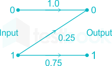
\(X \in \left{ { - a,; + a} \right}\) and

\(p\left( {X = a} \right) = p\left( {X = - a} \right) = 0.5\) 

\(Z \sim N\left( {\beta X,;1} \right)\);

Y = X + Z

There are two cases for Y:

1. When X = a, Y = a + Z

Since:

\(Z \sim N\left( {\beta a,;1} \right)\) 

\(Y \sim N\left( {a + \beta a,1} \right) = N\left( {a\left( {1 + \beta } \right),1} \right)\) 

\({f_Y}\left( {\frac{y}{{X = a}}} \right) = \frac{1}{{\sqrt {2\pi } }}{e^{ - \frac{{{{\left( {y - a\left( {1 + \beta } \right)} \right)}^2}}}{2}}}\) 

2. When X = -a, Y = a + Z

Since:

\(Z \sim N\left( { - \beta a,;1} \right)\) 

\(Y \sim N\left( { - a - \beta a,{\sigma ^2}} \right)\) 

\( = N\left( { - a\left( {1 + \beta } \right),1} \right)\) 

\({f_Y}\left( {\frac{y}{{X = - a}}} \right) = \frac{1}{{\sqrt {2\pi } }}{e^{ - \frac{{{{\left( {y + a\left( {1 + \beta } \right)} \right)}^2}}}{2}}}\)     

The probability of error will be:

\({P_e} = p\left( {x = a} \right) \times p\left( {\frac{e}{{x = a}}} \right) + p\left( {x = - a} \right) \times p\left( {\frac{e}{{x = - a}}} \right)\) 

Since a threshold detector with threshold 0 is used, we can write:

\({P_e} = p\left( {x = a} \right) \times p\left( {\frac{{y < 0}}{{x = a}}} \right) + p\left( {x = - a} \right) \times p\left( {\frac{{y > 0}}{{x = - a}}} \right)\) 

\( = 0.5 \times \mathop \smallint \nolimits_{ - \infty }^0 {f_Y}\left( {\frac{y}{{X = a}}} \right)dy + 0.5 \times \mathop \smallint \nolimits_0^\infty {f_Y}\left( {\frac{y}{{X = - a}}} \right)dy\)  

\( = 0.5 \times \mathop \smallint \nolimits_{ - \infty }^0 \frac{1}{{\sqrt {2\pi } }}{e^{ - \frac{{{{\left( {y - a\left( {1 + \beta } \right)} \right)}^2}}}{2}}}{\rm{;}}dy + 0.5 \times \mathop \smallint \nolimits_0^\infty \frac{1}{{\sqrt {2\pi } }}{e^{ - \frac{{{{\left( {y + a\left( {1 + \beta } \right)} \right)}^2}}}{2}}}dy\) 

Let u = y – a (1 + β) and v = y + a (1 + β)

du = dy and dv = dy

\({P_e} = 0.5 \times \mathop \smallint \nolimits_{ - \infty }^{ - a\left( {1 + \beta } \right)} \frac{1}{{\sqrt {2\pi } }}{e^{ - \frac{{{u^2}}}{2}}}{\rm{;}}du + 0.5 \times \mathop \smallint \nolimits_{a\left( {1 + \beta } \right)}^\infty \frac{1}{{\sqrt {2\pi } }}{e^{ - \frac{{{v^2}}}{2}}}dv\) 

Again, changing the variable of the first term, lets say u = -v

\({P_e} = 0.5 \times \mathop \smallint \nolimits_{a\left( {1 + \beta } \right)}^\infty \frac{1}{{\sqrt {2\pi } }}{e^{ - \frac{{{v^2}}}{2}}}{\rm{;}}dv + 0.5 \times \mathop \smallint \nolimits_{a\left( {1 + \beta } \right)}^\infty \frac{1}{{\sqrt {2\pi } }}{e^{ - \frac{{{v^2}}}{2}}}dv\) 

\({P_e} = \mathop \smallint \nolimits_{a\left( {1 + \beta } \right)}^\infty \frac{1}{{\sqrt {2\pi } }}{e^{ - \frac{{{v^2}}}{2}}}{\rm{;}}dv = Q\left( {a\left( {1 + \beta } \right)} \right)\) 

Given that when β = 0, then:

\({P_e} = Q\left( a \right) = {e^{ - \frac{{{a^2}}}{2}}} = 1 \times {10^{ - 8}}\) 

\(a = \sqrt {2 \times \ln \left( {{{10}^8}} \right)} \approx 6.07\) 

When β = -0.3 then:

\({P_e} = Q\left( {6.07 \times \left( {1 - 0.3} \right)} \right) = Q\left( {4.249} \right)\) 

\({P_e} \approx {e^{ - \frac{{{{4.249}^2}}}{2}}} \approx 1.2 \times {10^{ - 4}}\)

Concept:

The electrostatic potential difference between two points A and B is given by:

\({V_{AB}} = - \mathop \smallint \limits_A^B E \cdot dr\)

Analysis:

Given:

Point A: (0, 20 kV/cm)

Point B: (5 μm, 40 kV/cm)

Using the Equation of a line formula, we get:

\(\left( {E - 20} \right) = \frac{{40 - 20}}{{5 × {{10}^{ - 4}};cm - 0}}\left( {x - 0} \right)\)

E – 20 = 4 × 10⁴ x

E = (4 × 10⁴ x + 20) kV/cm

\({V_{AB}} = - \mathop \smallint \limits_A^B E \cdot dx\)

\(= - \left. {\mathop \smallint \limits_0^{5 × {{10}^{ - 4}}cm} \left( {4 × {{10}^4}x + 20} \right)dx = - \left( {2 × {{10}^4}{x^2} + 20x} \right)} \right|_0^{5 × {{10}^{ - 4}}}\)

\(= - \left( {2 × {{10}^4} × {{\left( {5 × {{10}^{ - 4}}} \right)}^2} + 20 × 5 × {{10}^{ - 4}}} \right);kV\)

= -(2 × 10⁴ × 25 × 10^-8 + 100 × 10^{^} - 4)kV

\(=-\left( 5\times {{10}^{-3}}+10\times {{10}^{-3}} \right)kV\)

= -15 × 10^-3 × 10³ V

V_AB = -15 V

Concept:

Stoke’s Theorem:

\(\mathop{\oint }_{C}A\cdot dt=\mathop{\int }_{S}\left( \nabla \times A \right)\cdot dt\)

Application:

Given:

\(\vec{F}=z{{\hat{a}}_{x}}+x~{{\hat{a}}_{y}}+y~{{\hat{a}}_{z}}\)

The sphre given is:

– x² + y² + z² = 1

\(\overrightarrow{dl}=dx~{{\hat{a}}_{x}}+dy~{{\hat{a}}_{y}}+dz~{{\hat{a}}_{z}}\)

\(\vec{F}\cdot \overrightarrow{dl}=\left( z\cdot {{{\hat{a}}}_{x}}+x~{{{\hat{a}}}_{y}}+y~{{{\hat{a}}}_{z}} \right)\cdot \left( {{d}_{x}}~{{{\hat{a}}}_{x}}+{{d}_{y}}~{{{\hat{a}}}_{y}}+dz~{{{\hat{a}}}_{z}} \right)\)

= z dx + x dy + y dz

Since interface is z = 0

Therefore, put z = 0 in \(\vec{F}\cdot \overrightarrow{dl}\) and the equation of the sphere, we get:

\(\vec{F}\cdot \overrightarrow{dl}=x~dy\)

x² + y² = 1

x = cos θ & y = sin θ

where θ ∈ [0, 2π]

\(\mathop{\int }_{S}\left( \nabla \times F \right)\cdot ds=\mathop{\oint }_{C}\vec{F}\cdot \overrightarrow{dl}\)

\(=\mathop{\oint }_{C}x~dy=\underset{\theta =0}{\overset{2\pi }{\mathop \int }},\cos \theta \times \left( \cos \theta ~d\theta \right)\)

\(=\underset{0}{\overset{2\pi }{\mathop \int }},{{\cos }^{2}}\theta ~d\theta \)

\(\left. =\underset{0}{\overset{2\pi }{\mathop \int }},\frac{\left( 1+\cos 20 \right)}{2}~d\theta =\frac{1}{2}\left( \theta +\frac{\sin 2\theta }{2} \right) \right|_{0}^{2\pi }\)

\(=\frac{1}{2}\times \left( 2\pi +\frac{\sin 4\pi }{2} \right)\)

\(=\frac{1}{2}\times \left( 2\pi -0 \right)\)

\(=\pi \simeq 3.14\)

Concept:

The electric field is related to the potential as:

\(\vec E = - ∇ V\)

\(∇ =\frac{\partial}{\partial x}\hat a_x+\frac{\partial}{\partial y}\hat a_y+\frac{\partial}{\partial z}\hat a_z\)

Calculation:

We can verify all options with the Maxwell equation \(\vec E = - ∇ V\)

Option 1: V = xy3 – yz2

\( - ∇ V=-(\frac{\partial}{\partial x} (xy^3 – yz^2)\hat a_x+\frac{\partial}{\partial y}(xy^3 – yz^2)\hat a_y+\frac{\partial}{\partial z}(xy^3 – yz^2)\hat a_z)\)

= -y³ a_x - (3xy² - z²) a_y - 2yz a_z

Since this is not equal to the given Electric field, this cannot be a valid expression for the given electrostatic potential.

Option 2: V = 2xy3 – xyz2

\( - ∇ V=-(\frac{\partial}{\partial x} (2xy^3 – xyz^2)\hat a_x+\frac{\partial}{\partial y}(2xy^3 – xyz^2)\hat a_y+\frac{\partial}{\partial z}(2xy^3 – xyz^2)\hat a_z)\)

= -[(2y3 - yz²) ax + (6xy2 - xz2) ay - 2xyz az]

Since this is not equal to the given Electric field, this cannot be a valid expression for the given electrostatic potential.

Option 3: V = y3 + xyz2

\( - ∇ V=-(\frac{\partial}{\partial x} (y^3 + xyz^2)\hat a_x+\frac{\partial}{\partial y}(y^3 + xyz^2)\hat a_y+\frac{\partial}{\partial z}(y^3 + xyz^2)\hat a_z)\)

= -[yz2 ax + (3y2 + xz2) ay + 2xyz az]

Since this is not equal to the given Electric field, this cannot be a valid expression for the given electrostatic potential.

Option 4: V = 2xy3 – 3xyz2

\( - ∇ V=-(\frac{\partial}{\partial x} (2xy^3 – 3xyz^2)\hat a_x+\frac{\partial}{\partial y}(2xy^3 – 3xyz^2)\hat a_y+\frac{\partial}{\partial z}(2xy^3 – 3xyz^2)\hat a_z)\)

= -[(2y³ - 3yz²)ax + (6xy2 - 3xz2) ay - 6xyz az]

= -(2y3 - 3yz2)ax - (6xy2 - 3xz2) ay + 6xyz az

Since E = - ∇ V for this case, this this is a valid expression for the given electrostatic potential.